Basic Statistical Methods

Configuring R

Functions from these packages will be used throughout this document:

library(conflicted) # check for conflicting function definitions
# library(printr) # inserts help-file output into markdown output
library(rmarkdown) # Convert R Markdown documents into a variety of formats.
library(pander) # format tables for markdown
library(ggplot2) # graphics
library(ggfortify) # help with graphics
library(dplyr) # manipulate data
library(tibble) # `tibble`s extend `data.frame`s
library(magrittr) # `%>%` and other additional piping tools
library(haven) # import Stata files
library(knitr) # format R output for markdown
library(tidyr) # Tools to help to create tidy data
library(plotly) # interactive graphics
library(dobson) # datasets from Dobson and Barnett 2018
library(parameters) # format model output tables for markdown
library(haven) # import Stata files
library(latex2exp) # use LaTeX in R code (for figures and tables)
library(fs) # filesystem path manipulations
library(survival) # survival analysis
library(survminer) # survival analysis graphics
library(KMsurv) # datasets from Klein and Moeschberger
library(parameters) # format model output tables for
library(webshot2) # convert interactive content to static for pdf
library(forcats) # functions for categorical variables ("factors")
library(stringr) # functions for dealing with strings
library(lubridate) # functions for dealing with dates and times
library(broom) # Summarizes key information about statistical objects in tidy tibbles
library(broom.helpers) # Provides suite of functions to work with regression model 'broom::tidy()' tibbles

Here are some R settings I use in this document:

rm(list = ls()) # delete any data that's already loaded into R

conflicts_prefer(dplyr::filter)
ggplot2::theme_set(
  ggplot2::theme_bw() + 
        # ggplot2::labs(col = "") +
    ggplot2::theme(
      legend.position = "bottom",
      text = ggplot2::element_text(size = 12, family = "serif")))

knitr::opts_chunk$set(message = FALSE)
options('digits' = 6)

panderOptions("big.mark", ",")
pander::panderOptions("table.emphasize.rownames", FALSE)
pander::panderOptions("table.split.table", Inf)
conflicts_prefer(dplyr::filter) # use the `filter()` function from dplyr() by default
legend_text_size = 9
run_graphs = TRUE

Acknowledgements

This content is adapted from Vittinghoff et al. (2012), Chapter 3.

1 Introduction

This appendix reviews fundamental statistical methods that are prerequisites for the main content of this course. Most of this material should be familiar from Epi 202 and Epi 203.

Example dataset: HERS

Throughout this appendix we use the HERS dataset as a running example.

The “heart and estrogen/progestin study” (HERS) was a clinical trial of hormone therapy for prevention of recurrent heart attacks and death among 2,763 post-menopausal women with existing coronary heart disease (CHD) (Hulley et al. 1998).

The trial was conducted at 20 US clinical centers. Participants were randomized to receive either conjugated equine estrogens (0.625 mg/day) plus medroxyprogesterone acetate (2.5 mg/day) or a matching placebo (Hulley et al. 1998). Women were followed for an average of 4.1 years (Hulley et al. 1998).

The primary outcome was nonfatal myocardial infarction or CHD death (Hulley et al. 1998).

library(haven)
hers <- haven::read_dta(
  paste0(
    "https://regression.ucsf.edu/sites/g/files",
    "/tkssra6706/f/wysiwyg/home/data/hersdata.dta"
  )
)

2 Descriptive Statistics

See Vittinghoff et al. (2012), §3.2.

2.1 Summary statistics for continuous variables

Sample mean

Definition 1 (Sample mean) The sample mean of \(n\) observations \(x_1, \ldots, x_n\) is:

\[\bar{x} = \frac{1}{n} \sum_{i=1}^{n} x_i\]

Sample variance

Definition 2 (Sample variance) The sample variance is:

\[s^2 = \frac{1}{n-1} \sum_{i=1}^{n} (x_i - \bar{x})^2\]

The divisor \(n - 1\) (rather than \(n\)) makes \(s^2\) an unbiased estimator of the population variance \(\sigma^2\).

Sample standard deviation

Definition 3 (Sample standard deviation) The sample standard deviation is \(s = \sqrt{s^2}\). It is expressed in the same units as the original data, making it more interpretable than the variance.

Sample median

Definition 4 (Sample median) The sample median is the middle value when observations are sorted in ascending order. For \(n\) observations:

• If \(n\) is odd, the median is the \(\frac{n+1}{2}\)th order statistic.
• If \(n\) is even, the median is the average of the \(\frac{n}{2}\)th and \(\frac{n}{2}+1\)th order statistics.

The median is more robust to outliers than the mean.

Interquartile range

Definition 5 (Interquartile range) The interquartile range (IQR) is the difference between the 75th percentile (the third quartile, \(Q_3\)) and the 25th percentile (the first quartile, \(Q_1\)):

\[\text{IQR} = Q_3 - Q_1\]

Like the median, the IQR is robust to outliers.

2.2 Summary statistics for categorical variables

Sample proportion

Definition 6 (Sample proportion) For a binary outcome, the sample proportion of “successes” (coded as 1) is:

\[\hat{p} = \frac{k}{n}\]

where \(k\) is the number of successes and \(n\) is the total sample size.

2.3 Computing summary statistics in R

The tbl_summary() function from the gtsummary package produces formatted summary tables:

HERS baseline summary statistics

Example 1  

library(dplyr)
library(gtsummary)
library(haven)

hers |>
  mutate(
    HT = haven::as_factor(HT),
    exercise = haven::as_factor(exercise),
    smoking = haven::as_factor(smoking),
    diabetes = haven::as_factor(diabetes)
  ) |>
  select(age, BMI, glucose, SBP, DBP, HT, exercise, smoking, diabetes) |>
  tbl_summary(
    by = HT,
    statistic = list(
      gtsummary::all_continuous() ~ "{mean} ({sd})",
      gtsummary::all_categorical() ~ "{n} ({p}%)"
    ),
    digits = gtsummary::all_continuous() ~ 1,
    label = list(
      age ~ "Age (years)",
      BMI ~ "BMI (kg/m²)",
      glucose ~ "Fasting glucose (mg/dL)",
      SBP ~ "Systolic BP (mmHg)",
      DBP ~ "Diastolic BP (mmHg)",
      exercise ~ "Exercises regularly",
      smoking ~ "Current smoker",
      diabetes ~ "Diabetes"
    )
  ) |>
  add_overall() |>
  bold_labels()

Table 1

Characteristic	Overall N = 2,7631	0 N = 1,3831	1 N = 1,3801
Age (years)	66.6 (6.7)	66.8 (6.7)	66.5 (6.6)
BMI (kg/m²)	28.6 (5.5)	28.5 (5.5)	28.6 (5.5)
Unknown	5	4	1
Fasting glucose (mg/dL)	112.2 (36.8)	112.4 (36.8)	111.9 (36.9)
Systolic BP (mmHg)	135.1 (19.0)	135.1 (19.4)	135.0 (18.7)
Diastolic BP (mmHg)	73.2 (9.7)	73.1 (9.7)	73.2 (9.7)
Unknown	1	1	0
Exercises regularly
0	1,695 (61%)	853 (62%)	842 (61%)
1	1,068 (39%)	530 (38%)	538 (39%)
Current smoker
0	2,403 (87%)	1,201 (87%)	1,202 (87%)
1	360 (13%)	182 (13%)	178 (13%)
Diabetes
0	2,032 (74%)	1,031 (75%)	1,001 (73%)
1	731 (26%)	352 (25%)	379 (27%)
1 Mean (SD); n (%)

2.4 Exploratory data analysis

Graphical summaries reveal aspects of the data distribution that summary statistics may miss, such as skewness, multimodality, and outliers.

Histograms

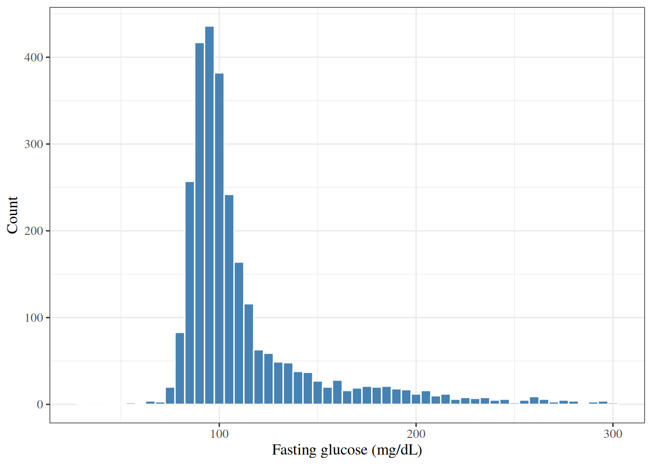
A histogram displays the distribution of a continuous variable by dividing the range of values into intervals (bins) and plotting the number or proportion of observations in each bin.

Distribution of fasting glucose

Example 2  

library(ggplot2)

hers |>
  ggplot() +
  aes(x = glucose) +
  geom_histogram(binwidth = 5, fill = "steelblue", color = "white") +
  labs(
    x = "Fasting glucose (mg/dL)",
    y = "Count"
  )

Figure 1: Distribution of fasting glucose (mg/dL) in HERS participants

Boxplots

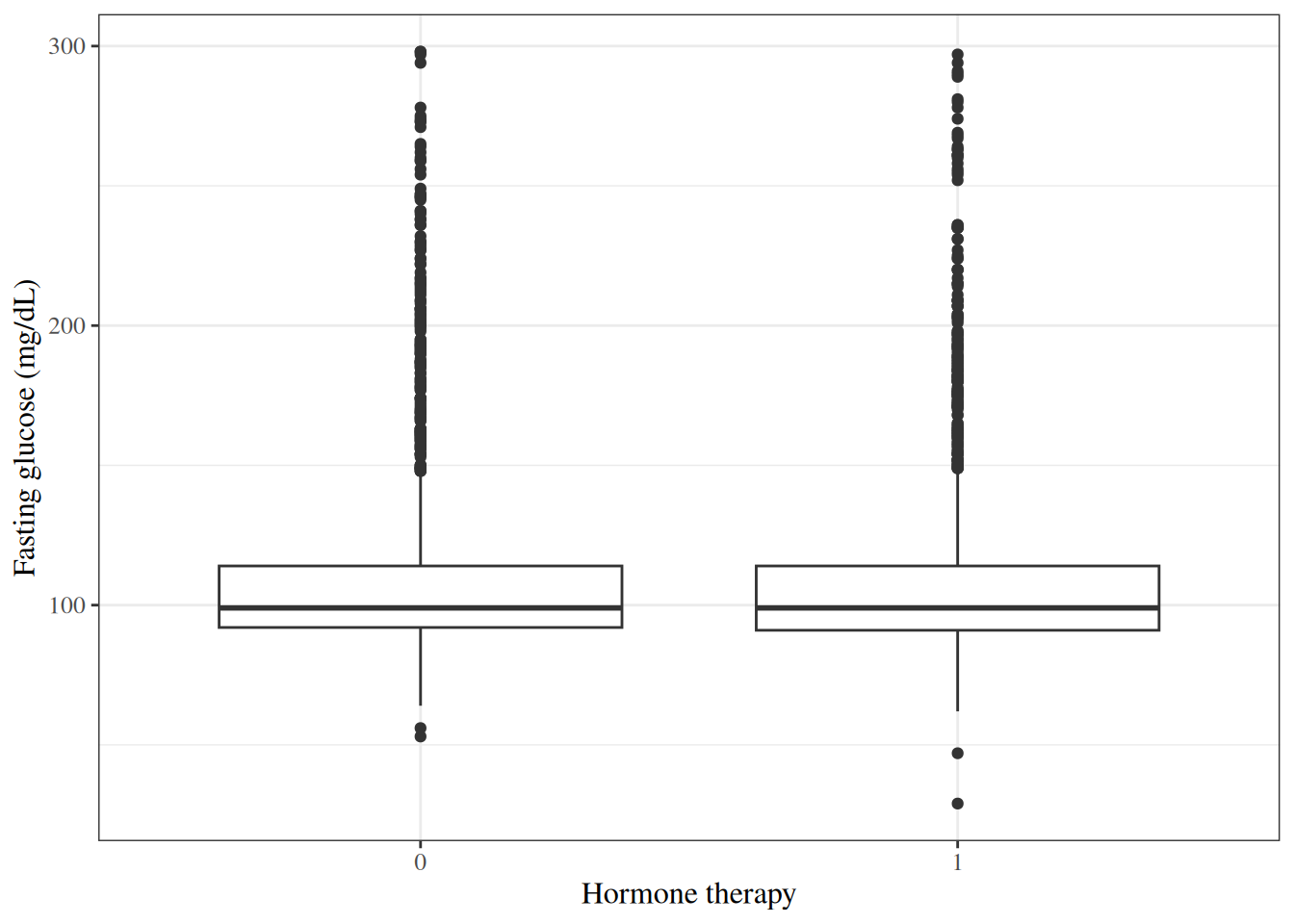
A boxplot (box-and-whisker plot) summarizes the distribution of a continuous variable using five statistics: the minimum, the first quartile (\(Q_1\)), the median, the third quartile (\(Q_3\)), and the maximum (with outliers plotted separately).

Fasting glucose by hormone therapy group

Example 3  

hers |>
  mutate(HT = haven::as_factor(HT)) |>
  ggplot() +
  aes(x = HT, y = glucose) +
  geom_boxplot() +
  labs(
    x = "Hormone therapy",
    y = "Fasting glucose (mg/dL)"
  )

Figure 2: Fasting glucose by hormone therapy assignment in HERS

Scatterplots

A scatterplot displays the joint distribution of two continuous variables by plotting each observation as a point.

BMI versus fasting glucose

Example 4  

hers |>
  ggplot() +
  aes(x = BMI, y = glucose) +
  geom_point(alpha = 0.3) +
  geom_smooth(method = "lm", se = TRUE) +
  labs(
    x = "BMI (kg/m²)",
    y = "Fasting glucose (mg/dL)"
  )

Figure 3: Fasting glucose versus BMI in HERS participants

3 Comparing Two Groups: Continuous Outcomes

See Vittinghoff et al. (2012), §3.3.

3.1 Hypotheses

Null hypothesis

Definition 7 (Null hypothesis) The null hypothesis \(H_0\) is a specific claim about the population parameter(s) that we test against the data. In a two-group comparison of means, the null hypothesis is typically that the two group means are equal:

\[H_0: \mu_1 = \mu_2\]

Alternative hypothesis

Definition 8 (Alternative hypothesis) The alternative hypothesis \(H_1\) (or \(H_A\)) is the claim we are trying to find evidence for. For a two-sided test:

\[H_1: \mu_1 \neq \mu_2\]

3.2 The two-sample t-test

Definition

Definition 9 (Two-sample t-test) The two-sample t-test (Welch’s t-test) tests whether the means of two independent groups are equal.

For samples of sizes \(n_1\) and \(n_2\) from two groups with sample means \(\bar{x}_1\), \(\bar{x}_2\) and sample variances \(s_1^2\), \(s_2^2\), the test statistic is:

\[t = \frac{\bar{x}_1 - \bar{x}_2}{\sqrt{\dfrac{s_1^2}{n_1} + \dfrac{s_2^2}{n_2}}}\]

Under \(H_0\), this statistic follows (approximately) a \(t\)-distribution with degrees of freedom estimated by the Welch-Satterthwaite equation.

Welch’s t-test vs. pooled t-test

Note

Welch’s t-test (the default in R’s t.test()) does not assume equal variances across groups. The pooled t-test assumes equal variances (\(\sigma_1^2 = \sigma_2^2\)) and pools the two sample variances into a single estimate. Welch’s t-test is generally preferred because the equal-variance assumption is rarely verifiable in practice (Vittinghoff et al. 2012, sec. 3.3).

Comparing fasting glucose between hormone therapy groups

Example 5 We test \(H_0: \mu_\text{placebo} = \mu_\text{HT}\) vs. \(H_1: \mu_\text{placebo} \neq \mu_\text{HT}\).

glucose_placebo <- hers |> filter(HT == 0) |> pull(glucose)
glucose_HT      <- hers |> filter(HT == 1) |> pull(glucose)

t.test(glucose_HT, glucose_placebo)
#> 
#>  Welch Two Sample t-test
#> 
#> data:  glucose_HT and glucose_placebo
#> t = -0.4246, df = 2761, p-value = 0.671
#> alternative hypothesis: true difference in means is not equal to 0
#> 95 percent confidence interval:
#>  -3.34503  2.15423
#> sample estimates:
#> mean of x mean of y 
#>   111.854   112.449

3.3 One-sample t-test

Definition

Definition 10 (One-sample t-test) The one-sample t-test tests whether the mean of a single population equals a specified null value \(\mu_0\):

\[H_0: \mu = \mu_0 \qquad H_1: \mu \neq \mu_0\]

The test statistic is:

\[t = \frac{\bar{x} - \mu_0}{s / \sqrt{n}}\]

Under \(H_0\), \(t \sim t_{n-1}\) (a t-distribution with \(n-1\) degrees of freedom).

3.4 Paired t-test

Definition

Definition 11 (Paired t-test) The paired t-test compares two related measurements (e.g., pre- and post-treatment values from the same subjects). Let \(d_i = x_{i,1} - x_{i,2}\) be the within-subject difference; the test reduces to a one-sample t-test on the differences:

\[H_0: \mu_d = 0 \qquad H_1: \mu_d \neq 0\]

Change in glucose over follow-up

Example 6  

# glucose1 is follow-up glucose; glucose is baseline
t.test(hers$glucose1, hers$glucose, paired = TRUE)
#> 
#>  Paired t-test
#> 
#> data:  hers$glucose1 and hers$glucose
#> t = 4.151, df = 2612, p-value = 3.42e-05
#> alternative hypothesis: true mean difference is not equal to 0
#> 95 percent confidence interval:
#>  1.38248 3.85824
#> sample estimates:
#> mean difference 
#>         2.62036

3.5 Confidence intervals for the difference in means

A two-sided \((1-\alpha) \cdot 100\%\) confidence interval for \(\mu_1 - \mu_2\) is:

\[(\bar{x}_1 - \bar{x}_2) \pm t^*_{df} \cdot \sqrt{\frac{s_1^2}{n_1} + \frac{s_2^2}{n_2}}\]

where \(t^*_{df}\) is the appropriate critical value from the t-distribution. The confidence interval is returned by t.test() in R alongside the hypothesis test result.

For more on confidence intervals, see Statistical Inference.

4 One-Way Analysis of Variance

Analysis of variance (ANOVA) generalizes the two-sample t-test to compare means across \(k \geq 2\) groups.

4.1 Definition

Definition 12 (One-way ANOVA) In a one-way ANOVA, we test:

\[H_0: \mu_1 = \mu_2 = \cdots = \mu_k\]

vs. the alternative that at least one mean differs.

The F-statistic compares the between-group variance to the within-group variance:

\[F = \frac{\text{MS}_\text{between}}{\text{MS}_\text{within}} = \frac{\text{SS}_\text{between}/(k-1)}{\text{SS}_\text{within}/(n-k)}\]

Under \(H_0\), \(F \sim F_{k-1, n-k}\).

Fasting glucose by race/ethnicity

Example 7  

aov_result <- aov(glucose ~ factor(raceth), data = hers)
summary(aov_result)
#>                  Df  Sum Sq Mean Sq F value  Pr(>F)    
#> factor(raceth)    2   45919   22959    17.1 4.1e-08 ***
#> Residuals      2760 3704543    1342                    
#> ---
#> Signif. codes:  0 '***' 0.001 '**' 0.01 '*' 0.05 '.' 0.1 ' ' 1

ANOVA as a special case of linear regression

Note

One-way ANOVA is equivalent to a linear regression model with a single categorical predictor. See Linear Models Overview for details.

5 Comparing Two Groups: Categorical Outcomes

See Vittinghoff et al. (2012), §3.5.

5.1 Contingency tables

Definition

Definition 13 (Contingency table) A contingency table (cross-tabulation) displays the joint frequencies of two categorical variables. For two binary variables, this is a \(2 \times 2\) table with cells \(a\), \(b\), \(c\), \(d\):

	Outcome = 1	Outcome = 0	Total
Exposure = 1	\(a\)	\(b\)	\(a + b\)
Exposure = 0	\(c\)	\(d\)	\(c + d\)
Total	\(a + c\)	\(b + d\)	\(n\)

Exercise by hormone therapy group

Example 8  

hers |>
  mutate(
    HT = haven::as_factor(HT),
    exercise = haven::as_factor(exercise)
  ) |>
  gtsummary::tbl_cross(
    row = exercise,
    col = HT,
    label = list(
      exercise ~ "Exercises regularly",
      HT ~ "Hormone therapy"
    ),
    percent = "row"
  )

Table 2: Exercise by hormone therapy group in HERS

	Hormone therapy		Total
	0	1
Exercises regularly
0	853 (50%)	842 (50%)	1,695 (100%)
1	530 (50%)	538 (50%)	1,068 (100%)
Total	1,383 (50%)	1,380 (50%)	2,763 (100%)

5.2 The chi-square test

Definition

Definition 14 (Chi-square test) The Pearson chi-square test tests whether two categorical variables are independent. For a \(2 \times 2\) table, the test statistic is:

\[\chi^2 = \sum_{i,j} \frac{(O_{ij} - E_{ij})^2}{E_{ij}}\]

where \(O_{ij}\) is the observed cell count and \(E_{ij} = \frac{(\text{row total}) \times (\text{column total})}{n}\) is the expected cell count under independence.

Under \(H_0\) (independence), \(\chi^2 \sim \chi^2_1\) for a \(2 \times 2\) table.

Chi-square test: exercise vs. hormone therapy

Example 9  

chisq.test(hers$exercise, hers$HT)
#> 
#>  Pearson's Chi-squared test with Yates' continuity correction
#> 
#> data:  hers$exercise and hers$HT
#> X-squared = 0.1016, df = 1, p-value = 0.75

5.3 Fisher’s exact test

Definition

Definition 15 (Fisher’s exact test) Fisher’s exact test computes the exact probability of observing a \(2 \times 2\) table at least as extreme as the observed table, given the marginal totals and under the null hypothesis of independence.

It is preferred over the chi-square test when cell counts are small (typically when any expected cell count is less than 5).

Fisher’s exact test example

Example 10  

fisher.test(hers$exercise, hers$HT)
#> 
#>  Fisher's Exact Test for Count Data
#> 
#> data:  hers$exercise and hers$HT
#> p-value = 0.725
#> alternative hypothesis: true odds ratio is not equal to 1
#> 95 percent confidence interval:
#>  0.879664 1.202192
#> sample estimates:
#> odds ratio 
#>    1.02836

5.4 Measures of association for 2×2 tables

See Odds Ratios and Relative Risks for definitions and formulas.

6 Correlation

See Vittinghoff et al. (2012), §3.6.

6.1 Pearson correlation coefficient

Definition

Definition 16 (Pearson correlation coefficient) The Pearson correlation coefficient measures the strength and direction of the linear association between two continuous variables \(X\) and \(Y\):

\[r = \frac{\sum_{i=1}^{n} (x_i - \bar{x})(y_i - \bar{y})} {\sqrt{\sum_{i=1}^{n}(x_i - \bar{x})^2 \sum_{i=1}^{n}(y_i - \bar{y})^2}}\]

\(r\) ranges from \(-1\) (perfect negative linear relationship) to \(+1\) (perfect positive linear relationship); \(r = 0\) indicates no linear association.

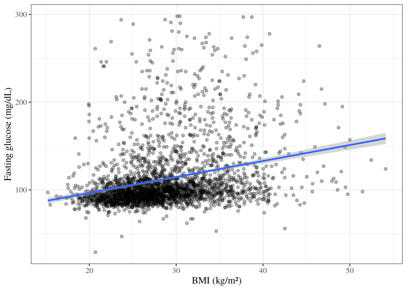
Correlation between BMI and glucose

Example 11  

cor.test(hers$BMI, hers$glucose, method = "pearson")
#> 
#>  Pearson's product-moment correlation
#> 
#> data:  hers$BMI and hers$glucose
#> t = 14.88, df = 2756, p-value <2e-16
#> alternative hypothesis: true correlation is not equal to 0
#> 95 percent confidence interval:
#>  0.237760 0.306865
#> sample estimates:
#>      cor 
#> 0.272664

6.2 Spearman rank correlation

Definition

Definition 17 (Spearman rank correlation) The Spearman rank correlation \(r_S\) is the Pearson correlation computed on the ranks of the observations. It measures the strength and direction of any monotone association (not just linear) and is more robust to outliers.

Spearman correlation between BMI and glucose

Example 12  

cor.test(hers$BMI, hers$glucose, method = "spearman")
#> 
#>  Spearman's rank correlation rho
#> 
#> data:  hers$BMI and hers$glucose
#> S = 2.33e+09, p-value <2e-16
#> alternative hypothesis: true rho is not equal to 0
#> sample estimates:
#>      rho 
#> 0.333751

7 Simple Linear Regression

See Vittinghoff et al. (2012), §3.6 and Linear Models Overview.

7.1 Model specification

Definition

Definition 18 (Simple linear regression) A simple linear regression model relates a continuous outcome \(Y\) to a single predictor \(X\):

\[Y_i = \beta_0 + \beta_1 x_i + \varepsilon_i, \qquad \varepsilon_i \overset{\text{iid}}{\sim} \operatorname{N}\mathopen{}\left(0, \sigma^2\right)\mathclose{}\]

• \(\beta_0\) is the intercept: the expected value of \(Y\) when \(X = 0\).
• \(\beta_1\) is the slope: the expected change in \(Y\) per one-unit increase in \(X\).
• \(\varepsilon_i\) are independent Gaussian errors with mean 0 and variance \(\sigma^2\).

7.2 Ordinary least squares estimation

The parameters \(\beta_0\) and \(\beta_1\) are estimated by minimizing the residual sum of squares (RSS):

\[\text{RSS} = \sum_{i=1}^n (y_i - \hat{y}_i)^2 = \sum_{i=1}^n (y_i - \hat\beta_0 - \hat\beta_1 x_i)^2\]

The closed-form ordinary least squares (OLS) estimators are:

\[\hat\beta_1 = r \cdot \frac{s_y}{s_x}, \qquad \hat\beta_0 = \bar{y} - \hat\beta_1 \bar{x}\]

where \(r\) is the Pearson correlation and \(s_x\), \(s_y\) are the sample standard deviations.

7.3 Fitting a simple linear regression in R

Glucose on BMI

Example 13  

Table 3

slr_fit <- lm(glucose ~ BMI, data = hers)
summary(slr_fit)
#> 
#> Call:
#> lm(formula = glucose ~ BMI, data = hers)
#> 
#> Residuals:
#>    Min     1Q Median     3Q    Max 
#> -81.55 -18.98 -10.35   3.76 190.81 
#> 
#> Coefficients:
#>             Estimate Std. Error t value Pr(>|t|)    
#> (Intercept)   60.074      3.565    16.9   <2e-16 ***
#> BMI            1.822      0.122    14.9   <2e-16 ***
#> ---
#> Signif. codes:  0 '***' 0.001 '**' 0.01 '*' 0.05 '.' 0.1 ' ' 1
#> 
#> Residual standard error: 35.5 on 2756 degrees of freedom
#>   (5 observations deleted due to missingness)
#> Multiple R-squared:  0.0743, Adjusted R-squared:  0.074 
#> F-statistic:  221 on 1 and 2756 DF,  p-value: <2e-16

The estimated slope is \(\hat\beta_1 = 1.82\) mg/dL per kg/m², meaning fasting glucose increases by approximately 1.82 mg/dL for each 1 kg/m² increase in BMI.

7.4 The coefficient of determination (\(R^2\))

Definition

Definition 19 (Coefficient of determination (\(R^2\))) The coefficient of determination \(R^2\) measures the proportion of the total variance in \(Y\) that is explained by the linear regression on \(X\):

\[R^2 = 1 - \frac{\text{RSS}}{\text{TSS}} = 1 - \frac{\sum_i (y_i - \hat{y}_i)^2}{\sum_i (y_i - \bar{y})^2}\]

\(R^2\) ranges from 0 (no linear relationship) to 1 (perfect linear fit). For simple linear regression, \(R^2 = r^2\).

7.5 Further reading

For a more thorough treatment of linear regression, see Linear Models Overview and Vittinghoff et al. (2012), Chapters 4 and 9.

8 Bootstrap Confidence Intervals

Adapted from (Vittinghoff et al. 2012, sec. 3.6, pp. 62–63).

8.1 When to use the bootstrap

Bootstrapping is a widely applicable method for obtaining standard errors and CIs in three situations:

• Approximate methods for computing valid CIs have been developed but are not conveniently implemented in standard software.
• Developing closed-form approximate methods has turned out to be intractable.
• The dataset violates the assumptions underlying established methods badly enough that the resulting CIs would be unreliable.

8.2 The bootstrap procedure

Definition 20 (Bootstrap sample) A bootstrap sample is a sample of size \(n\) drawn with replacement from the observed data of size \(n\). Because sampling is with replacement, each bootstrap sample contains some observations more than once and omits others entirely.

Example 14 (Bootstrap sample) Consider a dataset of five observations: \(\{3,\;7,\;5,\;2,\;9\}\) (\(n = 5\)). Two possible bootstrap samples drawn with replacement are:

Bootstrap sample	Values drawn	Notes
1	\(3,\;3,\;7,\;5,\;9\)	3 appears twice; 2 not drawn
2	\(2,\;7,\;7,\;9,\;5\)	7 appears twice; 3 not drawn

Each sample has size \(n = 5\) but may repeat or omit individual observations from the original dataset.

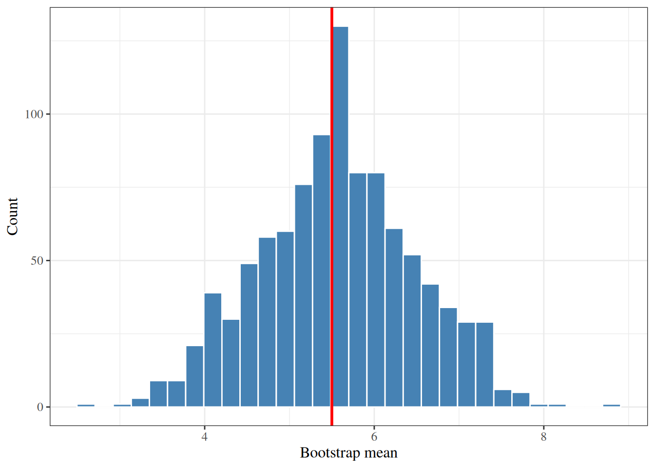
Definition 21 (Bootstrap distribution) The bootstrap distribution of a statistic is the empirical distribution of that statistic computed across a large number \(B\) of bootstrap samples. It serves as an estimate of the sampling distribution of the statistic. The bootstrap standard error is the standard deviation of the bootstrap distribution.

Example 15 (Bootstrap distribution)  

set.seed(42)
toy <- c(3, 7, 5, 2, 9, 4, 8, 1, 6, 10)
boot_means_toy <- replicate(
  1000,
  mean(sample(toy, replace = TRUE))
)
boot_se_toy <- sd(boot_means_toy)
boot_ci_norm_lo <- mean(toy) - 1.96 * boot_se_toy
boot_ci_norm_hi <- mean(toy) + 1.96 * boot_se_toy
boot_ci_perc <- quantile(boot_means_toy, c(0.025, 0.975))

Using the 10-observation dataset \(\mathopen{}\left\{3, 7, 5, 2, 9, 4, 8, 1, 6, 10\right\}\mathclose{}\) (observed mean 5.5), we draw \(B = 1{,}000\) bootstrap resamples and compute the sample mean of each. The bootstrap distribution is centered near the observed mean with bootstrap standard error 0.92.

library(ggplot2)
ggplot(data.frame(mean = boot_means_toy)) +
  aes(x = mean) +
  geom_histogram(bins = 30, color = "white", fill = "steelblue") +
  geom_vline(xintercept = mean(toy), color = "red", linewidth = 1) +
  labs(x = "Bootstrap mean", y = "Count")

Figure 4: Bootstrap distribution of the sample mean (\(B = 1{,}000\) replicates, \(n = 10\) toy dataset). The red line marks the observed mean (5.5). The distribution is approximately normal and centered near \(\bar{x}\).

The key idea is to treat the observed sample as a stand-in for the source population, and to mimic repeated sampling from that population by resampling with replacement from the observed data.

8.3 Bootstrap CI methods

Three methods for constructing a CI from the bootstrap distribution are in common use (Vittinghoff et al. 2012, sec. 3.6, p. 63):

Normal approximation

If the bootstrap distribution of the statistic of interest is approximately normal, replace the model-based standard error in a conventional CI with the bootstrap standard deviation:

\[\hat\theta \pm z^* \cdot \widehat{\text{SE}}_{\text{boot}}\]

This method requires fewer bootstrap replicates than percentile-based methods, but is less reliable when the sampling distribution departs from normality, particularly in the tails.

Example 16 (Normal approximation) Continuing from Example 15: the observed mean is 5.5 and the bootstrap standard error is 0.92. The 95% normal-approximation CI is:

\[\bar{x} \pm 1.96 \cdot \widehat{\text{SE}}_{\text{boot}}\]

which here evaluates to (3.71, 7.29).

Percentile method

The CI is constructed from the empirical quantiles of the bootstrap distribution. A 95% CI spans the 2.5th to 97.5th percentiles of the \(B\) bootstrap estimates.

Because the extreme percentiles of a finite sample are noisy estimates of the corresponding population quantiles, a larger number of replicates is required (typically \(B \geq 1{,}000\)).

Example 17 (Percentile method) Continuing from Example 15 with \(B = 1{,}000\) bootstrap means: the 2.5th percentile is 3.8 and the 97.5th percentile is 7.3, giving a 95% CI of (3.8, 7.3).

Bias-corrected and accelerated (BCa) method

The BCa interval adjusts the percentile-based CI to account for both bias (a shift between the observed statistic and the median of the bootstrap distribution) and skewness in the bootstrap distribution (James et al. 2021, chap. 5, p. 209). BCa intervals are preferred when the bootstrap distribution is noticeably skewed.

Example 18 (Bias-corrected and accelerated method) The BCa interval for the toy dataset is computed automatically by boot.ci() in R, which handles the bias-correction and acceleration adjustments internally. The comprehensive worked example below demonstrates all three CI methods side by side, making it straightforward to compare the BCa interval to the normal and percentile intervals.

8.4 Bootstrap CI in R

The boot package (included with base R) provides boot() for resampling and boot.ci() for all three CI types.

Bootstrap CI for the slope of SBP on age

Example 19 We adapt the example from (Vittinghoff et al. 2012, sec. 3.6, p. 62): a simple linear regression of systolic blood pressure (SBP) on age in the HERS dataset.

library(boot)

# statistic function: returns the slope of SBP ~ age
boot_slope <- function(data, indices) {
  fit <- lm(SBP ~ age, data = data[indices, ])
  coef(fit)[["age"]]
}

set.seed(42)
boot_result <- boot(
  data = hers,
  statistic = boot_slope,
  R = 1000
)

boot_result
#> 
#> ORDINARY NONPARAMETRIC BOOTSTRAP
#> 
#> 
#> Call:
#> boot(data = hers, statistic = boot_slope, R = 1000)
#> 
#> 
#> Bootstrap Statistics :
#>     original       bias    std. error
#> t1* 0.471728 -0.000635537   0.0536514

The bootstrap standard error closely matches the model-based standard error from lm(). All three bootstrap intervals below are consistent with the parametric CI.

boot.ci(
  boot_result,
  type = c("norm", "perc", "bca")
)
#> BOOTSTRAP CONFIDENCE INTERVAL CALCULATIONS
#> Based on 1000 bootstrap replicates
#> 
#> CALL : 
#> boot.ci(boot.out = boot_result, type = c("norm", "perc", "bca"))
#> 
#> Intervals : 
#> Level      Normal             Percentile            BCa          
#> 95%   ( 0.3672,  0.5775 )   ( 0.3607,  0.5811 )   ( 0.3624,  0.5824 )  
#> Calculations and Intervals on Original Scale

The normal, percentile, and BCa intervals are all similar here, consistent with the bootstrap distribution being approximately symmetric. In cases with more skewness, the BCa interval would differ more from the others, and should be preferred.

Hulley, Stephen, Deborah Grady, Trudy Bush, et al. 1998. “Randomized Trial of Estrogen Plus Progestin for Secondary Prevention of Coronary Heart Disease in Postmenopausal Women.” JAMA : The Journal of the American Medical Association (Chicago, IL) 280 (7): 605–13.

James, Gareth, Daniela Witten, Trevor Hastie, and Robert Tibshirani. 2021. An Introduction to Statistical Learning: With Applications in R. 2nd ed. Springer. https://doi.org/10.1007/978-1-0716-1418-1.

Vittinghoff, Eric, David V Glidden, Stephen C Shiboski, and Charles E McCulloch. 2012. Regression Methods in Biostatistics: Linear, Logistic, Survival, and Repeated Measures Models. 2nd ed. Springer. https://doi.org/10.1007/978-1-4614-1353-0.