Linear (Gaussian) Models

Configuring R

Functions from these packages will be used throughout this document:

[R code]
library(conflicted) # check for conflicting function definitions
# library(printr) # inserts help-file output into markdown output
library(rmarkdown) # Convert R Markdown documents into a variety of formats.
library(pander) # format tables for markdown
library(ggplot2) # graphics
library(ggfortify) # help with graphics
library(dplyr) # manipulate data
library(tibble) # `tibble`s extend `data.frame`s
library(magrittr) # `%>%` and other additional piping tools
library(haven) # import Stata files
library(knitr) # format R output for markdown
library(tidyr) # Tools to help to create tidy data
library(plotly) # interactive graphics
library(dobson) # datasets from Dobson and Barnett 2018
library(parameters) # format model output tables for markdown
library(haven) # import Stata files
library(latex2exp) # use LaTeX in R code (for figures and tables)
library(fs) # filesystem path manipulations
library(survival) # survival analysis
library(survminer) # survival analysis graphics
library(KMsurv) # datasets from Klein and Moeschberger
library(parameters) # format model output tables for
library(webshot2) # convert interactive content to static for pdf
library(forcats) # functions for categorical variables ("factors")
library(stringr) # functions for dealing with strings
library(lubridate) # functions for dealing with dates and times
library(broom) # Summarizes key information about statistical objects in tidy tibbles
library(broom.helpers) # Provides suite of functions to work with regression model 'broom::tidy()' tibbles

Here are some R settings I use in this document:

[R code]
rm(list = ls()) # delete any data that's already loaded into R

conflicts_prefer(dplyr::filter)
ggplot2::theme_set(
  ggplot2::theme_bw() + 
        # ggplot2::labs(col = "") +
    ggplot2::theme(
      legend.position = "bottom",
      text = ggplot2::element_text(size = 12, family = "serif")))

knitr::opts_chunk$set(message = FALSE)
options('digits' = 6)

panderOptions("big.mark", ",")
pander::panderOptions("table.emphasize.rownames", FALSE)
pander::panderOptions("table.split.table", Inf)
conflicts_prefer(dplyr::filter) # use the `filter()` function from dplyr() by default
legend_text_size = 9
run_graphs = TRUE
[R code]
include_reference_lines <- FALSE

Note

This content is adapted from:

  • Dobson and Barnett (2018), Chapters 2-6
  • Dunn and Smyth (2018), Chapters 2-3
  • Vittinghoff et al. (2012), Chapter 4

There are numerous textbooks specifically for linear regression, including:

  • Kutner et al. (2005): used for UCLA Biostatistics MS level linear models class
  • Chatterjee and Hadi (2015): used for Stanford MS-level linear models class
  • Seber and Lee (2012): used for UCLA Biostatistics PhD level linear models class and UC Davis STA 108.
  • Kleinbaum et al. (2014): same first author as Kleinbaum and Klein (2010) and Kleinbaum and Klein (2012)
  • Linear Models with R (Faraway 2025)
  • Applied Linear Regression by Sanford Weisberg (Weisberg 2005)

For more recommendations, see the discussion on Reddit.

1 Overview

1.1 Why this course includes linear regression

  • This course is about generalized linear models (for non-Gaussian outcomes)
  • UC Davis STA 108 (“Applied Statistical Methods: Regression Analysis”) is a prerequisite for this course, so everyone here should have some understanding of linear regression already.
  • We will review linear regression to:
  • make sure everyone is caught up
  • provide an epidemiological perspective on model interpretation.

1.2 Chapter overview

  • Section 2: how to interpret linear regression models

  • Section 3: how to estimate linear regression models

  • Section 4: how to tell if your model is insufficiently complex

  • Section 5: how to quantify uncertainty about our estimates and generate predictions

2 Understanding Gaussian Linear Regression Models

2.1 General form of a Gaussian linear regression model

Definition 1 (General form of a Gaussian linear regression model) A Gaussian linear regression model has two components:

  1. The random part

    (the outcome distribution model):

    \[ Y_i|\tilde{x}_i \ \sim_{\perp\!\!\!\perp}\ \operatorname{N}(\mu_i,\sigma^2) \]

    Here \(\tilde{x}_i\) is the observed covariate vector for unit \(i\). Here \(\ \sim_{\perp\!\!\!\perp}\ \) means independently distributed. Conditional on \(\tilde{x}_1,\ldots,\tilde{x}_n\), the responses are independent across units, and each \(Y_i|\tilde{x}_i\) follows the same conditional distributional form with common variance \(\sigma^2\) while allowing \(\mu_i\) to vary by observation.

  2. The systematic part

    (the linear predictor component):

    \[ \begin{aligned} \mu_i &= \tilde{\beta} \cdot \tilde{x}_i \\ &= \beta_0 + \beta_1 x_{i1} + \cdots + \beta_p x_{ip} \end{aligned} \]

2.2 Motivating example: birthweights and gestational age

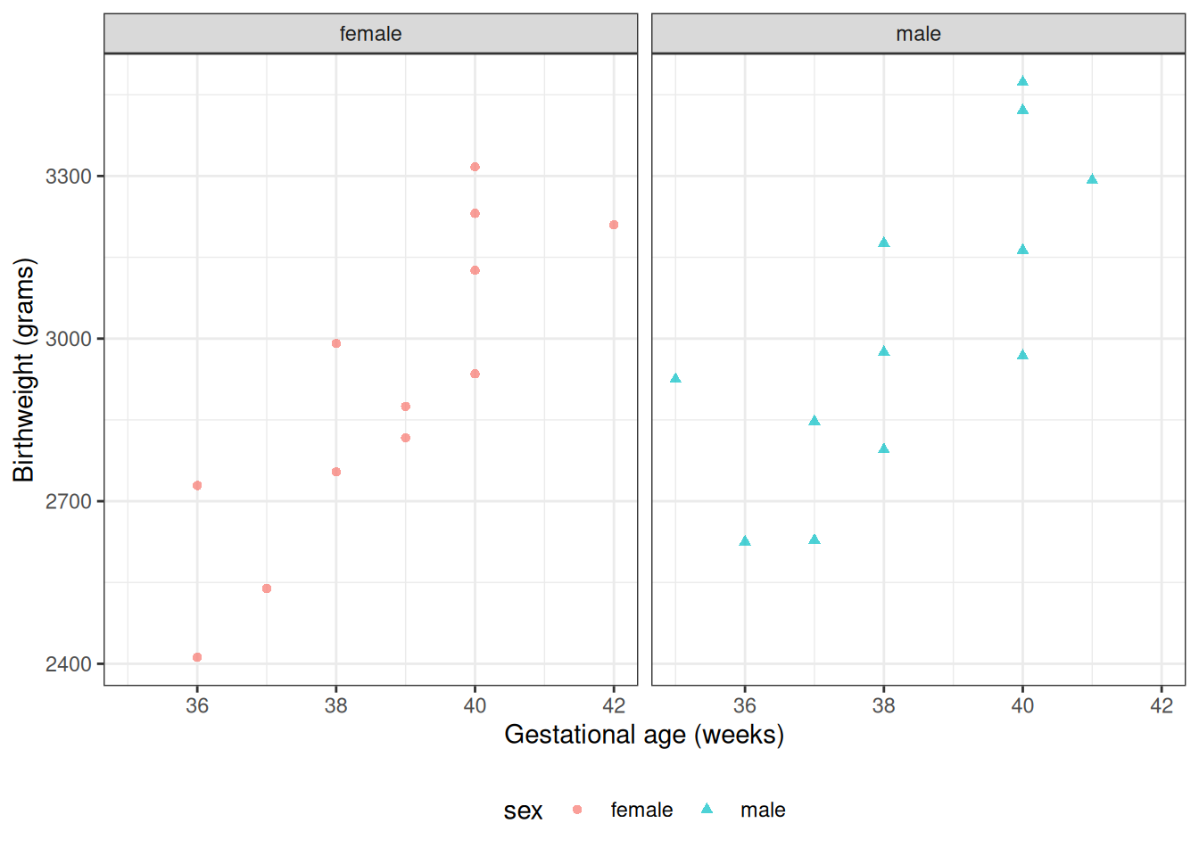
Suppose we want to learn about the distributions of birthweights (outcome \(Y\)) for (human) babies born at different gestational ages (covariate \(A\)) and with different chromosomal sexes (covariate \(S\)) (Dobson and Barnett (2018) Example 2.2.2).

2.3 Dobson birthweight data

Data as table

[R code]
library(dobson)
data("birthweight", package = "dobson")
birthweight
Table 1: birthweight data (Dobson and Barnett (2018) Example 2.2.2)

Reshape data for graphing

[R code]
library(tidyverse)
bw <-
  birthweight |>
  pivot_longer(
    cols = everything(),
    names_to = c("sex", ".value"),
    names_sep = "s "
  ) |>
  rename(age = `gestational age`) |>
  mutate(
    id = row_number(),
    sex = sex |>
      case_match(
        "boy" ~ "male",
        "girl" ~ "female"
      ) |>
      factor(levels = c("female", "male")),
    male = sex == "male",
    female = sex == "female"
  )

bw
Table 2: birthweight data reshaped

Data as graph

[R code]
plot1 <- bw |>
  ggplot(aes(
    x = age,
    y = weight,
    shape = sex,
    col = sex
  )) +
  theme_bw() +
  xlab("Gestational age (weeks)") +
  ylab("Birthweight (grams)") +
  theme(legend.position = "bottom") +
  # expand_limits(y = 0, x = 0) +
  geom_point(alpha = .7)
print(plot1 + facet_wrap(~sex))
Figure 1: birthweight data (Dobson and Barnett (2018) Example 2.2.2)

Data notation

  • \(Y\): birthweight (measured in grams)
  • \(S\): chromosomal sex: “male” (XY) or “female” (XX)
  • \(M\): indicator variable for \(S\) = “male”1
    • \(M = 0\) if \(S\) = “female”
    • \(M = 1\) if \(S\) = “male”
  • \(F\): indicator variable for \(S\) = “female”2
    • \(F = 1\) if \(S\) = “female”
    • \(F = 0\) if \(S\) = “male”
  • \(A\): estimated gestational age at birth (measured in weeks).

2.4 Parallel lines regression

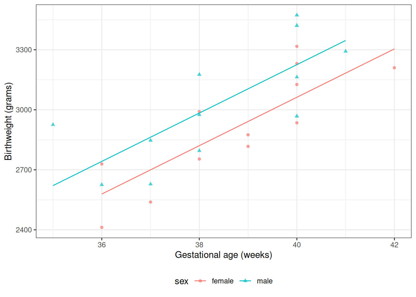
\[ \begin{aligned} Y|M,A &\ \sim_{\operatorname{ciid}}\ N(\mu(M,A), \sigma^2)\\ \mu(m,a) &= \beta_0 + \beta_M m + \beta_A a \end{aligned} \tag{1}\]

[R code]
bw_lm1 <- lm(
  formula = weight ~ sex + age,
  data = bw
)

library(parameters)
bw_lm1 |>
  parameters::parameters() |>
  parameters::print_md(
    include_reference = include_reference_lines,
    select = "{estimate}"
  )
Table 3: Regression parameter estimates for Model 1 of birthweight data
Parameter Coefficient
(Intercept) -1773.32
sex (male) 163.04
age 120.89
[R code]
bw <-
  bw |>
  mutate(`E[Y|X=x]` = fitted(bw_lm1)) |>
  arrange(sex, age)

plot2 <-
  plot1 %+% bw +
  geom_line(aes(y = `E[Y|X=x]`))

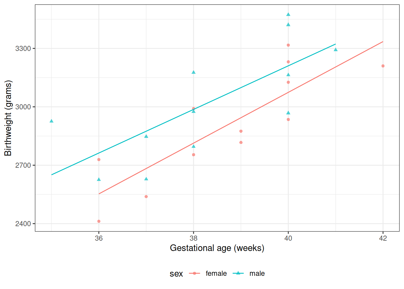
print(plot2)
Figure 2: Graph of Model 1 for birthweight data

Model assumptions and predictions

Exercise 1 What’s the mean birthweight for a female born at 36 weeks?

Estimated coefficients for model 1
Parameter Coefficient
(Intercept) -1773.32
sex (male) 163.04
age 120.89

Solution.  

Estimated coefficients for model 1
Parameter Coefficient
(Intercept) -1773.32
sex (male) 163.04
age 120.89
[R code]
pred_female <- coef(bw_lm1)["(Intercept)"] + coef(bw_lm1)["age"] * 36
## or using built-in prediction:
pred_female_alt <- predict(bw_lm1, newdata = tibble(sex = "female", age = 36))

\[ \begin{aligned} E[Y|M = 0, A = 36] &= \beta_0 + \mathopen{}\left(\beta_M \cdot 0\right)\mathclose{}+ \mathopen{}\left(\beta_A \cdot 36\right)\mathclose{} \\ &= -1773.321839 + \mathopen{}\left(163.039303 \cdot 0\right)\mathclose{} + \mathopen{}\left(120.894327 \cdot 36\right)\mathclose{} \\ &= 2578.873934 \end{aligned} \]

Exercise 2 What’s the mean birthweight for a male born at 36 weeks?

Estimated coefficients for model 1
Parameter Coefficient
(Intercept) -1773.32
sex (male) 163.04
age 120.89

Solution.  

Estimated coefficients for model 1
Parameter Coefficient
(Intercept) -1773.32
sex (male) 163.04
age 120.89
[R code]
pred_male <-
  coef(bw_lm1)["(Intercept)"] +
  coef(bw_lm1)["sexmale"] +
  coef(bw_lm1)["age"] * 36

\[ \begin{aligned} E[Y|M = 1, A = 36] &= \beta_0 + \beta_M \cdot 1+ \beta_A \cdot 36 \\ &= 2741.913237 \end{aligned} \]

Exercise 3 What’s the difference in mean birthweights between males born at 36 weeks and females born at 36 weeks?

[R code]
coef(bw_lm1)
#> (Intercept)     sexmale         age 
#>   -1773.322     163.039     120.894

Solution. \[ \begin{aligned} & E[Y|M = 1, A = 36] - E[Y|M = 0, A = 36]\\ &= 2741.913237 - 2578.873934\\ &= 163.039303 \end{aligned} \]

Shortcut:

\[ \begin{aligned} & E[Y|M = 1, A = 36] - E[Y|M = 0, A = 36]\\ &= (\beta_0 + \beta_M \cdot 1+ \beta_A \cdot 36) - (\beta_0 + \beta_M \cdot 0+ \beta_A \cdot 36) \\ &= \beta_M \\ &= 163.039303 \end{aligned} \]

Coefficient Interpretation

\[ E[Y|M=m,A=a] = \mu(m,a) = \beta_0 + \beta_M m + \beta_A a \]

Slope (of the mean with respect to age) for males: \[ \begin{aligned} \frac{d}{da}\mu(1,a) &= \frac{d}{da}(\beta_0 + \beta_M \cdot 1 + {\color{red}{\beta_A}} \cdot a)\\ &= \left(\frac{d}{da}\beta_0 + \frac{d}{da}\beta_M \cdot 1 + \frac{d}{da}({\color{red}{\beta_A}} \cdot a)\right)\\ &= (0 + 0 + {\color{red}{\beta_A}}) \\ &= {\color{red}{\beta_A}} \end{aligned} \]

Slope for females:

\[ \begin{aligned} \frac{d}{da}\mu(0,a) &= \frac{d}{da}(\beta_0 + \beta_M \cdot 0 + {\color{red}{\beta_A}} \cdot a)\\ &= \left(\frac{d}{da}\beta_0 + \frac{d}{da}\beta_M \cdot 0 + \frac{d}{da}({\color{red}{\beta_A}} \cdot a)\right)\\ &= (0 + 0 + {\color{red}{\beta_A}}) \\ &= {\color{red}{\beta_A}} \end{aligned} \]

Exercise 4 What is the interpretation of \(\beta_A\) in Model 1?

Solution. \[ \begin{aligned} \frac{d}{da}\mu(m,a) &= \frac{d}{da}(\beta_0 + \beta_M \cdot m + {\color{red}{\beta_A}} \cdot a)\\ &= \left(\frac{d}{da}\beta_0 + \frac{d}{da}\beta_M \cdot m + \frac{d}{da}({\color{red}{\beta_A}} \cdot a)\right)\\ &= (0 + 0 + {\color{red}{\beta_A}}) \\ &= {\color{red}{\beta_A}} \end{aligned} \]

Conclusion:

\[\beta_A = \frac{d}{da}\mu(m,a)\]

\[\beta_A = E[Y|M = m, A = a+1] - E[Y|M = m, A = a]\]

Exercise 5 What is the interpretation of \(\beta_M\) in Model 1?

Solution.

\[ \begin{aligned} E[Y|M = 1,A = a] &= \beta_0 + {\color{red}{\beta_M}} 1 + \beta_A a \\ & = \beta_0 + {\color{red}{\beta_M}} + \beta_A a \\ E[Y|M = 0,A = a] &= \beta_0 + {\color{red}{\beta_M}} 0 + \beta_A a \\ & = \beta_0 + \beta_A a \end{aligned} \] So: \[ \begin{aligned} E[Y|M = 1,A = a] - E[Y|M = 0,A = a] &= (\beta_0 + {\color{red}{\beta_M}} + \beta_A a) - (\beta_0 + \beta_A a) \\ &= {\color{red}{\beta_M}} \end{aligned} \] Therefore: \[ \begin{aligned} \beta_M &= E[Y|M = 1,A = a] - E[Y|M = 0,A = a]\\ & =\mu(1,a) - \mu(0,a)\\ \end{aligned} \]

In words: \(\beta_M\) is the difference in mean birthweight between males and females adjusting for age.

Exercise 6 \(\beta_0 = ?\)

Solution. \[ \begin{aligned} \operatorname{E}\mathopen{}\left[Y|M = 0,A = 0\right]\mathclose{} &= \mu(0,0)\\ &= {\color{red}{\beta_0}} + \beta_M 0 + \beta_A 0\\ &= {\color{red}{\beta_0}}\\ {\color{red}{\beta_0}} &= \operatorname{E}\mathopen{}\left[Y|M = 0,A = 0\right]\mathclose{} = \mu(0,0) \end{aligned} \]

2.5 Interactions

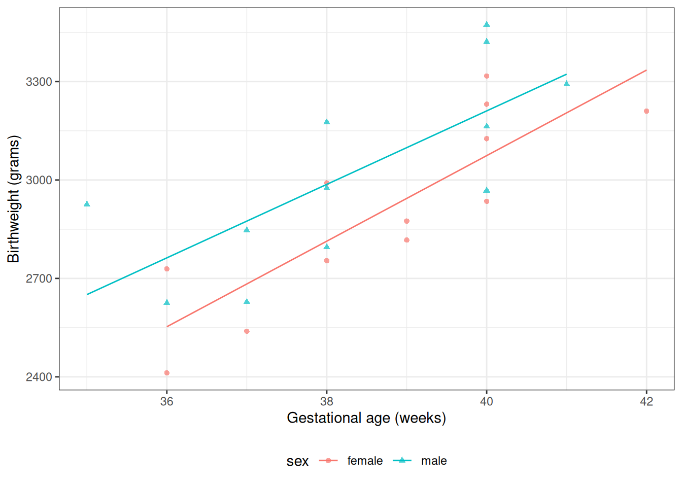
\[E[Y|S=s,A=a] = \beta_0 + \beta_A a+ \beta_M m + \beta_{AM} (a \cdot m) \tag{2}\]

[R code]
bw_lm2 <- lm(weight ~ sex + age + sex:age, data = bw)
bw_lm2 |>
  parameters() |>
  parameters::print_md(
    include_reference = include_reference_lines,
    select = "{estimate}"
  )
Table 4: Birthweight model with interaction term
Parameter Coefficient
(Intercept) -2141.67
sex (male) 872.99
age 130.40
sex (male) × age -18.42
[R code]
bw <-
  bw |>
  mutate(
    predlm2 = predict(bw_lm2)
  ) |>
  arrange(sex, age)

plot1_interact <-
  plot1 %+% bw +
  geom_line(aes(y = predlm2))

print(plot1_interact)
Figure 3: Birthweight model with interaction term

Here’s another way we could rewrite this model (by collecting terms involving \(S\)):

\[ E[Y|M,A] = \beta_0 + \beta_M M+ (\beta_A + \beta_{AM} M) A \]

Exercise 7 According to this model, what’s the mean birthweight for a female born at 36 weeks?

Parameter Coefficient
(Intercept) -2141.67
sex (male) 872.99
age 130.40
sex (male) × age -18.42

Solution.  

Parameter Coefficient
(Intercept) -2141.67
sex (male) 872.99
age 130.40
sex (male) × age -18.42
[R code]
pred_female <- coef(bw_lm2)["(Intercept)"] + coef(bw_lm2)["age"] * 36

\[ E[Y|M = 0, A = 36] = \beta_0 + \beta_M \cdot 0+ \beta_A \cdot 36 + \beta_{AM} \cdot (0 * 36) = 2552.733333 \]

Exercise 8 What’s the mean birthweight for a male born at 36 weeks?

Parameter Coefficient
(Intercept) -2141.67
sex (male) 872.99
age 130.40
sex (male) × age -18.42

Solution.  

Parameter Coefficient
(Intercept) -2141.67
sex (male) 872.99
age 130.40
sex (male) × age -18.42
[R code]
pred_male <-
  coef(bw_lm2)["(Intercept)"] +
  coef(bw_lm2)["sexmale"] +
  coef(bw_lm2)["age"] * 36 +
  coef(bw_lm2)["sexmale:age"] * 36

\[ \begin{aligned} E[Y|M = 1, A = 36] &= \beta_0 + \beta_M \cdot 1+ \beta_A \cdot 36 + \beta_{AM} \cdot 1 \cdot 36\\ &= 2762.706897 \end{aligned} \]

Exercise 9 What’s the difference in mean birthweights between males born at 36 weeks and females born at 36 weeks?

Solution. \[ \begin{aligned} & E[Y|M = 1, A = 36] - E[Y|M = 0, A = 36]\\ &= (\beta_0 + \beta_M \cdot 1+ \beta_A \cdot 36 + \beta_{AM} \cdot 1 \cdot 36)\\ &\ \ \ \ \ -(\beta_0 + \beta_M \cdot 0+ \beta_A \cdot 36 + \beta_{AM} \cdot 0 \cdot 36) \\ &= \beta_M + \beta_{AM}\cdot 36\\ &= 209.973563 \end{aligned} \]

Coefficient Interpretation

Exercise 10 What is the interpretation of \(\beta_{M}\) in Model 2?

Solution.  

Mean birthweight among males with gestational age 0 weeks: \[ \begin{aligned} \mu(1,0) &= \operatorname{E}\mathopen{}\left[Y|M = 1,A = 0\right]\mathclose{}\\ &= \beta_0 + {\color{red}{\beta_M}} \cdot 1 + \beta_A \cdot 0 + \beta_{AM}\cdot 1 \cdot 0\\ &= \beta_0 + {\color{red}{\beta_M}} \end{aligned} \] Mean birthweight among females with gestational age 0 weeks: \[ \begin{aligned} \mu(0,0) &= \operatorname{E}\mathopen{}\left[Y|M = 0,A = 0\right]\mathclose{}\\ &= \beta_0 + {\color{red}{\beta_M}} \cdot 0 + \beta_A \cdot 0 + \beta_{AM}\cdot 0 \cdot 0\\ &= \beta_0 \end{aligned} \]

\[ \begin{aligned} \beta_{M} &= \mu(1,0) - \mu(0,0) \\ &= \operatorname{E}\mathopen{}\left[Y|M = 1,A = 0\right]\mathclose{} - \operatorname{E}\mathopen{}\left[Y|M = 0,A = 0\right]\mathclose{} \end{aligned} \] \(\beta_M\) is the difference in mean birthweight between males with gestational age 0 weeks and females with gestational age 0 weeks.

Exercise 11 What is the interpretation of \(\beta_{AM}\) in Model 2?

Solution.  

Slope among males: \[ \begin{aligned} \frac{\partial}{\partial a}\mu(1,a) &= \frac{\partial}{\partial a}\left(\beta_0 + \beta_M\cdot1 + {\color{blue}{\beta_A}}\cdot a + {\color{red}{\beta_{AM}}}\cdot 1 \cdot a\right)\\ &= \frac{\partial}{\partial a}\left(\beta_0 + \beta_M + {\color{blue}{\beta_A}}\cdot a + {\color{red}{\beta_{AM}}} \cdot a\right)\\ &= {\color{blue}{\beta_A}} + {\color{red}{\beta_{AM}}} \end{aligned} \] or \[ \begin{aligned} E[Y|1,a+1] - E[Y|1,a] = &\beta_0 + \beta_M \cdot 1 + {\color{blue}{\beta_A}}\cdot(a+1) + {\color{red}{\beta_{AM}}} \cdot 1 \cdot (a+1)\\ &- (\beta_0 + \beta_M \cdot 1 + {\color{blue}{\beta_A}}\cdot a + {\color{red}{\beta_{AM}}} \cdot 1 \cdot a)\\ = &{\color{blue}{\beta_A}} + {\color{red}{\beta_{AM}}} \end{aligned} \]

Slope among females: \[ \begin{aligned} \frac{\partial}{\partial a}\mu(0,a) &= \frac{\partial}{\partial a}\left(\beta_0 + \beta_M\cdot0 + {\color{blue}{\beta_A}}\cdot a + {\color{red}{\beta_{AM}}}\cdot 0 \cdot a\right)\\ &= \frac{\partial}{\partial a}\left(\beta_0 + {\color{blue}{\beta_A}}\cdot a\right)\\ &= {\color{blue}{\beta_A}} \\ \end{aligned} \] or \[ \begin{aligned} E[Y|0,a+1] - E[Y|0,a] = &\beta_0 + \beta_M \cdot 0 + {\color{blue}{\beta_A}}\cdot(a+1) + {\color{red}{\beta_{AM}}} \cdot 0 \cdot (a+1) \\ &- (\beta_0 + \beta_M \cdot 0 + {\color{blue}{\beta_A}}\cdot a + {\color{red}{\beta_{AM}}} \cdot 0 \cdot a)\\ = &\beta_0 + {\color{blue}{\beta_A}}\cdot(a+1) - (\beta_0 + {\color{blue}{\beta_A}}\cdot a)\\ = &{\color{blue}{\beta_A}} \end{aligned} \]

Difference in slopes: \[ \begin{aligned} \frac{\partial}{\partial a}\mu(1,a) - \frac{\partial}{\partial a}\mu(0,a) &= {\color{blue}{\beta_A}} + {\color{red}{\beta_{AM}}} - {\color{blue}{\beta_A}}\\ &= {\color{red}{\beta_{AM}}} \end{aligned} \] or \[ \begin{aligned} (E[Y|1,a+1] - E[Y|1,a]) - (E[Y|0,a+1] - E[Y|0,a]) &= {\color{blue}{\beta_A}} + {\color{red}{\beta_{AM}}} - {\color{blue}{\beta_A}}\\ &= {\color{red}{\beta_{AM}}} \end{aligned} \]

Therefore \[ \begin{aligned} \beta_{AM} = &\frac{\partial}{\partial a}\mu(1,a) - \frac{\partial}{\partial a}\mu(0,a)\\ = &(E[Y|M = 1,A = a+1] - E[Y|M = 1,A = a])\\ &- (E[Y|M = 0,A = a+1] - E[Y|M = 0,A = a]) \end{aligned} \]

\(\beta_{AM}\) is the difference in slope of mean birthweight with respect to gestational age between males and females.

Compare coefficient interpretations

Table 5: Coefficient interpretations, by model structure
\(\mu(m,a)\) \(\beta_0 + \beta_M m + \beta_A a\) \(\beta_0 + \beta_M m + \beta_A a + {\color{red}{\beta_{AM} ma}}\)
\(\beta_0\) \(\mu(0,0)\) \(\mu(0,0)\)
\(\beta_A\) \(\frac{\partial}{\partial a}\mu({\color{blue}{m}},a)\) \(\frac{\partial}{\partial a}\mu({\color{red}{0}},a)\)
\(\beta_M\) \(\mu(1, {\color{blue}{a}}) - \mu(0, {\color{blue}{a}})\) \(\mu(1, {\color{red}{0}}) - \mu(0,{\color{red}{0}})\)
\(\beta_{AM}\) \(\frac{\partial}{\partial a}\mu(1,a) - \frac{\partial}{\partial a}\mu(0,a)\)

General procedure for interpreting coefficients

Definition 2 (General procedure for interpreting a regression coefficient) To derive the interpretation of coefficient \(\beta_j\) in a model with linear predictor \(\eta(\tilde{x}) = \eta(x_1, \ldots, x_p)\):

  1. Write down the linear predictor \(\eta(x_1, \ldots, x_p)\).

  2. Differentiate or difference \(\eta\) with respect to \(x_j\):

    1. If \(x_j\) is continuous: compute the partial derivative \(\frac{\partial}{\partial x_j}\eta(\tilde{x})\).

    2. If \(x_j\) is discrete: compute the one-unit difference \(\eta(\tilde{x})\big|_{x_j = a+1} - \eta(\tilde{x})\big|_{x_j = a}\).

    For an interaction coefficient \(\beta_{jk}\) (multiplying the product \(x_j \cdot x_k\)), apply this step twice in sequence: first differentiate or difference \(\eta\) with respect to \(x_j\) to obtain the slope of \(x_j\) as a function of \(x_k\); then differentiate or difference that slope with respect to \(x_k\) (choosing continuous/discrete as appropriate for \(x_k\)) to obtain the change in slopes, which equals \(\beta_{jk}\).

  3. If any covariates remain, set them to their reference levels. If covariates other than the one(s) used in step 2 still appear in the resulting expression, substitute each covariate’s reference level for it. This eliminates the corresponding interaction terms and isolates \(\beta_j\) alone on the right-hand side.

  4. Identify \(\beta_j\): the expression from the previous steps equals \(\beta_j\); write \(\beta_j = \cdots\) to state the interpretation explicitly.

Special case — intercept (\(\beta_0\)): If the coefficient of interest is the intercept \(\beta_0\), skip step 2. Apply step 3 directly by setting all covariates to their reference levels: \(\beta_0 = \eta(\text{reference pattern})\).

Example 1 (Applying the procedure to Model 1) For the birthweight parallel-lines model \[\operatorname{E}\mathopen{}\left[Y|M=m, A=a\right]\mathclose{} = \beta_0 + \beta_M m + \beta_A a,\] where \(M \in \{0,1\}\) (sex; \(1\) = male, \(0\) = female) and \(A\) is gestational age (weeks):

\(\beta_A\) (gestational age, continuous): \(\frac{\partial}{\partial a}\eta(m,a) = \beta_A\), so \(\beta_A = \frac{\partial}{\partial a}\operatorname{E}\mathopen{}\left[Y|M=m, A=a\right]\mathclose{}\). (Step 3 not needed: no remaining covariates appear after differentiating.)

\(\beta_M\) (sex, discrete):

\[ \begin{aligned} \eta(m,a)\big|_{m=1} - \eta(m,a)\big|_{m=0} &= (\beta_0 + \beta_M + \beta_A a) - (\beta_0 + \beta_A a) \\ &= \beta_M, \end{aligned} \]

so \(\beta_M = \operatorname{E}\mathopen{}\left[Y|M=1, A=a\right]\mathclose{} - \operatorname{E}\mathopen{}\left[Y|M=0, A=a\right]\mathclose{}\). (Step 3 not needed: \(a\) cancels in the differencing, so the result holds for all values of \(A\).)

\(\beta_0\) (intercept, special case): Skip step 2; set \(m=0\) and \(a=0\) (the reference levels) in step 3: \(\beta_0 = \eta(0,0) = \operatorname{E}\mathopen{}\left[Y|M=0, A=0\right]\mathclose{}\).

2.6 Stratified regression

\[ \operatorname{E}\mathopen{}\left[Y|A=a, S=s\right]\mathclose{} = \beta_M m + \beta_{AM} (a \cdot m) + \beta_F f + \beta_{AF} (a \cdot f) \tag{3}\]

Compare this stratified model (Equation 3) with our interaction model, Equation 2:

\[ \operatorname{E}\mathopen{}\left[Y|A=a, S=s\right]\mathclose{} = \beta_0 + \beta_A a + \beta_M m + \beta_{AM} (a \cdot m) \]

[R code]
bw_lm2 <- lm(weight ~ sex + age + sex:age, data = bw)
bw_lm2 |>
  parameters() |>
  print_md(
    include_reference = include_reference_lines,
    select = "{estimate}"
  )
Table 6: Birthweight model with interaction term
Parameter Coefficient
(Intercept) -2141.67
sex (male) 872.99
age 130.40
sex (male) × age -18.42
[R code]
bw_lm_strat <-
  bw |>
  lm(
    formula = weight ~ sex + sex:age - 1,
    data = _
  )

bw_lm_strat |>
  parameters() |>
  print_md(
    select = "{estimate}"
  )
Table 7: Birthweight model - stratified betas
Parameter Coefficient
sex (female) -2141.67
sex (male) -1268.67
sex (female) × age 130.40
sex (male) × age 111.98

2.7 Curved-line regression

[R code]
bw_lm3 <- lm(weight ~ sex:log(age) - 1, data = bw)

ggbw <-
  bw |>
  ggplot(
    aes(x = age, y = weight)
  ) +
  geom_point() +
  xlab("Gestational Age (weeks)") +
  ylab("Birth Weight (g)")

ggbw2 <- ggbw +
  stat_smooth(
    method = "lm",
    formula = y ~ log(x),
    geom = "smooth"
  ) +
  xlab("Gestational Age (weeks)") +
  ylab("Birth Weight (g)")


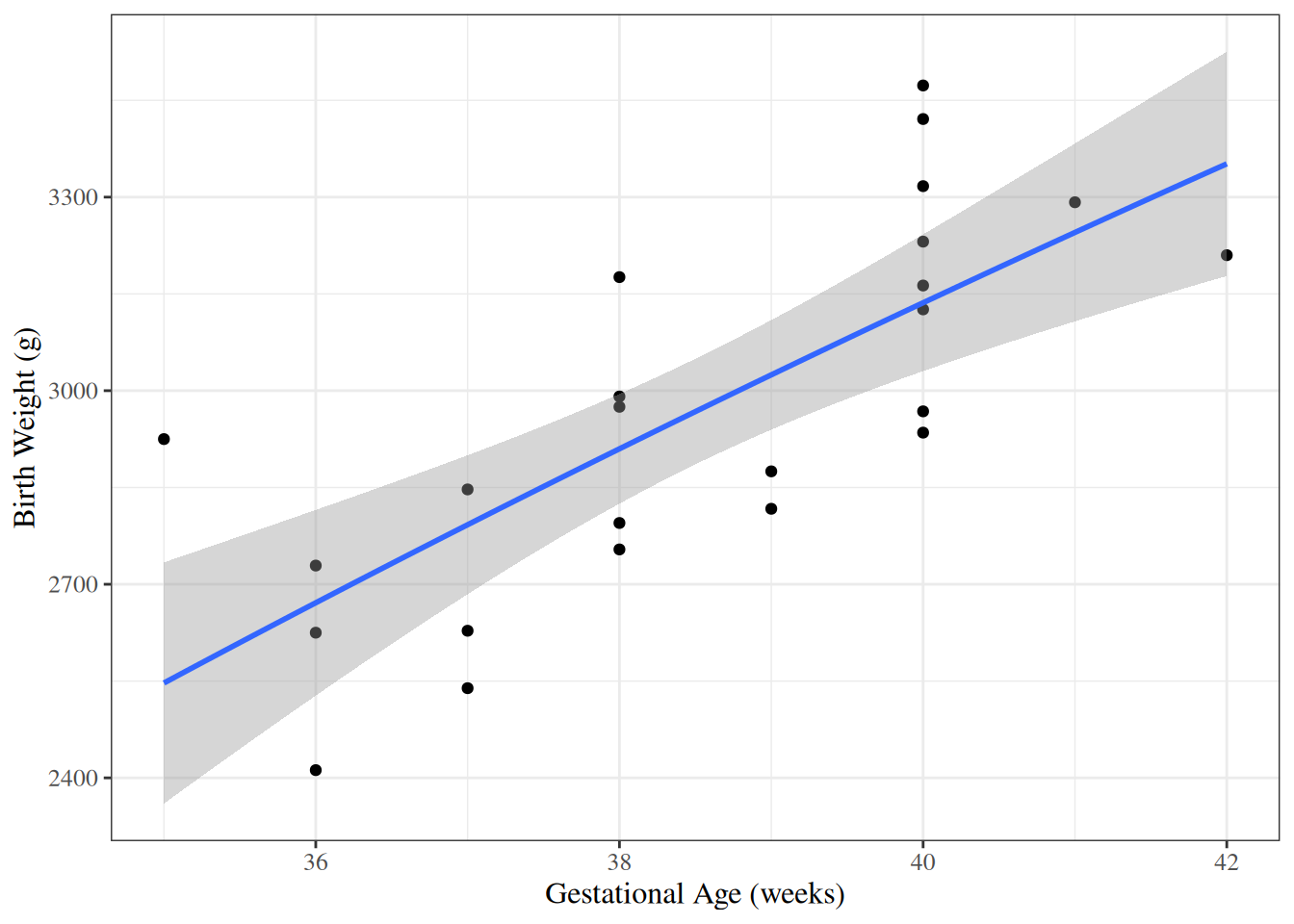
ggbw2 |> print()
Figure 4: birthweight model with age entering on log scale
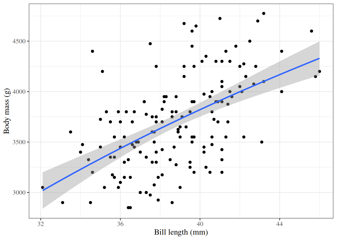
[R code]
library(palmerpenguins)

ggpenguins <-
  palmerpenguins::penguins |>
  dplyr::filter(species == "Adelie") |>
  ggplot(
    aes(x = bill_length_mm, y = body_mass_g)
  ) +
  geom_point() +
  xlab("Bill length (mm)") +
  ylab("Body mass (g)")

ggpenguins2 <- ggpenguins +
  stat_smooth(
    method = "lm",
    formula = y ~ log(x),
    geom = "smooth"
  ) +
  xlab("Bill length (mm)") +
  ylab("Body mass (g)")


ggpenguins2 |> print()
Figure 5: palmerpenguins model with bill_length entering on log scale

2.8 Rescaling

Rescale age

Exercise 12 Let \(A^* = A - 32\) weeks.

Consider a new version of Model 2, with \(A^*\) in place of \(A\):

\[ \operatorname{E}\mathopen{}\left[Y|M=m, A^*=a^*\right]\mathclose{} = \gamma_0 + \gamma_M m + \gamma_{A^*} a^* + \gamma_{A^*M} (m \cdot a^*) \tag{4}\]

Let the coefficients of this model be \(\gamma\)s instead of \(\beta\)s.

What are the interpretations of the \(\gamma\)s? How do they relate to the \(\beta\)s in Model 2? Which have the same interpretation? Which are different, and how do they differ? What is the pattern?

Solution. Interpretation of \(\gamma_0\):

From Model 4, \(\gamma_0\) is the mean birthweight among females (\(M = 0\)) with \(A^* = 0\) (i.e., \(A = 32\) weeks):

\[ \gamma_0 = \operatorname{E}\mathopen{}\left[Y|M=0, A^*=0\right]\mathclose{} = \operatorname{E}\mathopen{}\left[Y|M=0, A=32\right]\mathclose{} \]

Substituting into Model 2:

\[ \begin{aligned} \gamma_0 &= \beta_0 + \beta_M \cdot 0 + \beta_A \cdot 32 + \beta_{AM} \cdot 0 \cdot 32\\ &= \beta_0 + 32\beta_A \end{aligned} \]

This differs from \(\beta_0 = \operatorname{E}\mathopen{}\left[Y|M=0, A=0\right]\mathclose{}\), which is the mean birthweight among females at \(A = 0\) weeks.

Interpretation of \(\gamma_M\):

From Model 4, \(\gamma_M\) is the sex difference in mean birthweight at \(A^* = 0\) (i.e., \(A = 32\) weeks):

\[ \begin{aligned} \gamma_M &= \operatorname{E}\mathopen{}\left[Y|M=1, A^*=0\right]\mathclose{} - \operatorname{E}\mathopen{}\left[Y|M=0, A^*=0\right]\mathclose{}\\ &= \operatorname{E}\mathopen{}\left[Y|M=1, A=32\right]\mathclose{} - \operatorname{E}\mathopen{}\left[Y|M=0, A=32\right]\mathclose{} \end{aligned} \]

Substituting into Model 2:

\[ \begin{aligned} \gamma_M &= (\beta_0 + \beta_M + \beta_A \cdot 32 + \beta_{AM} \cdot 32) - (\beta_0 + \beta_A \cdot 32)\\ &= \beta_M + 32\beta_{AM} \end{aligned} \]

This differs from \(\beta_M\), which is the sex difference at \(A = 0\) weeks.

Interpretation of \(\gamma_{A^*}\):

From Model 4, \(\gamma_{A^*}\) is the slope of mean birthweight with respect to \(A^*\) among females (\(M = 0\)):

\[ \begin{aligned} \gamma_{A^*} &= \frac{d}{da^*}\operatorname{E}\mathopen{}\left[Y|M=0, A^*=a^*\right]\mathclose{}\\ &= \frac{d}{da^*}\operatorname{E}\mathopen{}\left[Y|M=0, A=a^*+32\right]\mathclose{}\\ &= \frac{d}{da}\operatorname{E}\mathopen{}\left[Y|M=0, A=a\right]\mathclose{} \end{aligned} \]

Substituting into Model 2:

\[ \begin{aligned} \gamma_{A^*} &= \frac{d}{da}\left(\beta_0 + \beta_A \cdot a\right)\\ &= \beta_A \end{aligned} \]

Since shifting \(A\) by a constant does not change the slope, \(\gamma_{A^*} = \beta_A\): these two coefficients have the same value and interpretation.

Interpretation of \(\gamma_{A^*M}\):

From Model 4, \(\gamma_{A^*M}\) is the difference in slope with respect to \(A^*\) between males and females:

\[ \begin{aligned} \gamma_{A^*M} &= \frac{d}{da^*}\operatorname{E}\mathopen{}\left[Y|M=1, A^*=a^*\right]\mathclose{} - \frac{d}{da^*}\operatorname{E}\mathopen{}\left[Y|M=0, A^*=a^*\right]\mathclose{}\\ &= \frac{d}{da}\operatorname{E}\mathopen{}\left[Y|M=1, A=a\right]\mathclose{} - \frac{d}{da}\operatorname{E}\mathopen{}\left[Y|M=0, A=a\right]\mathclose{} \end{aligned} \]

Substituting into Model 2:

\[ \begin{aligned} \gamma_{A^*M} &= (\beta_A + \beta_{AM}) - \beta_A\\ &= \beta_{AM} \end{aligned} \]

Since shifting \(A\) by a constant does not change slopes, \(\gamma_{A^*M} = \beta_{AM}\): these two coefficients have the same value and interpretation.

The pattern:

Slope coefficients (\(\gamma_{A^*}\) and \(\gamma_{A^*M}\)) are unchanged by rescaling: they have the same values and interpretations as the corresponding \(\beta\)s.

Coefficients change only for variables that have interactions with the rescaled variable \(A\). This includes the intercept (which can be viewed as the main effect of a variable that interacts with \(A\) via \(\beta_A\)), and the main effect of \(M\) (which interacts with \(A\) via \(\beta_{AM}\)). Shifting \(A\) by 32 weeks changes the reference point from \(A = 0\) to \(A = 32\), so these coefficients now represent quantities evaluated at \(A = 32\) weeks rather than at \(A = 0\) weeks.

Exercise 13 Using R, fit the rescaled interaction model with \(A^* = A - 36\) weeks in place of \(A\) in Model 2. Compare the coefficient estimates with those from the original model. Which coefficients change, and which remain the same?

Solution.

[R code]
bw <-
  bw |>
  mutate(
    `age - mean` = age - mean(age),
    `age - 36wks` = age - 36
  )

lm1_c <- lm(weight ~ sex + `age - 36wks`, data = bw)

lm2_c <- lm(weight ~ sex + `age - 36wks` + sex:`age - 36wks`, data = bw)

parameters(lm2_c, ci_method = "wald") |> print_md()
Parameter Coefficient SE 95% CI t(20) p
(Intercept) 2552.73 97.59 (2349.16, 2756.30) 26.16 < .001
sex (male) 209.97 129.75 (-60.68, 480.63) 1.62 0.121
age - 36wks 130.40 30.00 (67.82, 192.98) 4.35 < .001
sex (male) × age - 36wks -18.42 41.76 (-105.52, 68.68) -0.44 0.664

Compare with what we got without rescaling:

[R code]
parameters(bw_lm2, ci_method = "wald") |> print_md()
Parameter Coefficient SE 95% CI t(20) p
(Intercept) -2141.67 1163.60 (-4568.90, 285.56) -1.84 0.081
sex (male) 872.99 1611.33 (-2488.18, 4234.17) 0.54 0.594
age 130.40 30.00 (67.82, 192.98) 4.35 < .001
sex (male) × age -18.42 41.76 (-105.52, 68.68) -0.44 0.664

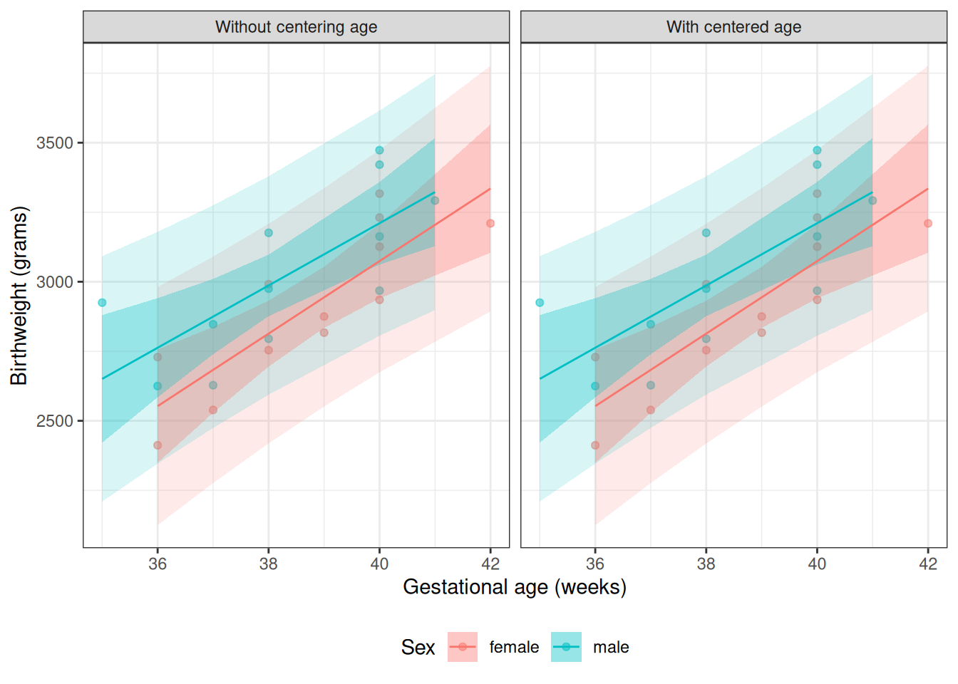
Centering gestational age does not change predictions

Centering gestational age changes the coefficient parameterization, but it does not change fitted values, confidence bands, or prediction bands.

The next output reports maximum absolute differences between the uncentered and centered models. All values should be near zero (up to floating-point rounding), which confirms that centering changes parameterization only.

[R code]
bw_centered <-
  bw |>
  dplyr::mutate(
    age_mean_centered = age - mean(age)
  )

bw_lm2_centered <-
  lm(
    weight ~ sex + age_mean_centered + sex:age_mean_centered,
    data = bw_centered
  )

pred_uncentered_ci <-
  predict(
    bw_lm2,
    newdata = bw_centered,
    interval = "confidence"
  ) |>
  tibble::as_tibble()

pred_centered_ci <-
  predict(
    bw_lm2_centered,
    newdata = bw_centered,
    interval = "confidence"
  ) |>
  tibble::as_tibble()

pred_uncentered_pi <-
  predict(
    bw_lm2,
    newdata = bw_centered,
    interval = "predict"
  ) |>
  tibble::as_tibble()

pred_centered_pi <-
  predict(
    bw_lm2_centered,
    newdata = bw_centered,
    interval = "predict"
  ) |>
  tibble::as_tibble()

tibble::tibble(
  fitted_max_abs_diff = max(abs(pred_uncentered_ci$fit - pred_centered_ci$fit)),
  ci_lwr_max_abs_diff = max(abs(pred_uncentered_ci$lwr - pred_centered_ci$lwr)),
  ci_upr_max_abs_diff = max(abs(pred_uncentered_ci$upr - pred_centered_ci$upr)),
  pi_lwr_max_abs_diff = max(abs(pred_uncentered_pi$lwr - pred_centered_pi$lwr)),
  pi_upr_max_abs_diff = max(abs(pred_uncentered_pi$upr - pred_centered_pi$upr))
)
[R code]
comparison_plot_data <-
  dplyr::bind_rows(
    bw_centered |>
      dplyr::bind_cols(
        pred_uncentered_ci |>
          dplyr::transmute(
            fit,
            ci_lwr = lwr,
            ci_upr = upr
          ),
        pred_uncentered_pi |>
          dplyr::transmute(
            pred_lwr = lwr,
            pred_upr = upr
          )
      ) |>
      dplyr::transmute(
        age,
        weight,
        sex,
        model = "Without centering age",
        fit,
        ci_lwr,
        ci_upr,
        pred_lwr,
        pred_upr
      ),
    bw_centered |>
      dplyr::bind_cols(
        pred_centered_ci |>
          dplyr::transmute(
            fit,
            ci_lwr = lwr,
            ci_upr = upr
          ),
        pred_centered_pi |>
          dplyr::transmute(
            pred_lwr = lwr,
            pred_upr = upr
          )
      ) |>
      dplyr::transmute(
        age,
        weight,
        sex,
        model = "With centered age",
        fit,
        ci_lwr,
        ci_upr,
        pred_lwr,
        pred_upr
      )
  ) |>
  dplyr::mutate(
    model = factor(
      model,
      levels = c("Without centering age", "With centered age")
    )
  )

comparison_plot_data |>
  ggplot2::ggplot(
    ggplot2::aes(
      x = age,
      y = weight,
      col = sex,
      fill = sex,
      group = sex
    )
  ) +
  ggplot2::geom_point(alpha = 0.5) +
  ggplot2::geom_ribbon(
    ggplot2::aes(
      ymin = pred_lwr,
      ymax = pred_upr
    ),
    alpha = 0.15,
    col = NA
  ) +
  ggplot2::geom_ribbon(
    ggplot2::aes(
      ymin = ci_lwr,
      ymax = ci_upr
    ),
    alpha = 0.3,
    col = NA
  ) +
  ggplot2::geom_line(
    ggplot2::aes(y = fit)
  ) +
  ggplot2::facet_wrap(~model) +
  ggplot2::theme_bw() +
  ggplot2::theme(legend.position = "bottom") +
  ggplot2::labs(
    x = "Gestational age (weeks)",
    y = "Birthweight (grams)",
    col = "Sex",
    fill = "Sex"
  )
Figure 6: Two-panel comparison of the fitted birthweight model bw_lm2 with and without centering gestational age, showing identical fitted values, confidence bands, and prediction bands in both panels.

2.9 Categorical covariates with more than two levels

Example: birthweight

In the birthweight example, the variable sex had only two observed values:

[R code]
unique(bw$sex)
#> [1] female male  
#> Levels: female male

If there are more than two observed values, we can’t just use a single variable with 0s and 1s.

Example: iris

[R code]
head(iris)
Table 8: The iris data
[R code]
library(table1)
table1(
  x = ~ . | Species,
  data = iris,
  overall = FALSE
)
Table 9: Summary statistics for the iris data
setosa
(N=50)
versicolor
(N=50)
virginica
(N=50)
Sepal.Length
Mean (SD) 5.01 (0.352) 5.94 (0.516) 6.59 (0.636)
Median [Min, Max] 5.00 [4.30, 5.80] 5.90 [4.90, 7.00] 6.50 [4.90, 7.90]
Sepal.Width
Mean (SD) 3.43 (0.379) 2.77 (0.314) 2.97 (0.322)
Median [Min, Max] 3.40 [2.30, 4.40] 2.80 [2.00, 3.40] 3.00 [2.20, 3.80]
Petal.Length
Mean (SD) 1.46 (0.174) 4.26 (0.470) 5.55 (0.552)
Median [Min, Max] 1.50 [1.00, 1.90] 4.35 [3.00, 5.10] 5.55 [4.50, 6.90]
Petal.Width
Mean (SD) 0.246 (0.105) 1.33 (0.198) 2.03 (0.275)
Median [Min, Max] 0.200 [0.100, 0.600] 1.30 [1.00, 1.80] 2.00 [1.40, 2.50]

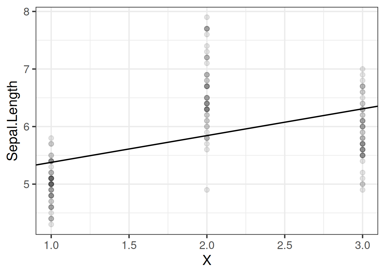
If we want to model Sepal.Length by species, we could create a variable \(X\) that represents “setosa” as \(X=1\), “virginica” as \(X=2\), and “versicolor” as \(X=3\).

[R code]
data(iris) # this step is not always necessary, but ensures you're starting
# from the original version of a dataset stored in a loaded package

iris <-
  iris |>
  tibble() |>
  mutate(
    X = case_when(
      Species == "setosa" ~ 1,
      Species == "virginica" ~ 2,
      Species == "versicolor" ~ 3
    )
  )

iris |>
  distinct(Species, X)
Table 10: iris data with numeric coding of species

Then we could fit a model like:

[R code]
iris_lm1 <- lm(Sepal.Length ~ X, data = iris)
iris_lm1 |>
  parameters() |>
  print_md()
Table 11: Model of iris data with numeric coding of Species
Parameter Coefficient SE 95% CI t(148) p
(Intercept) 4.91 0.16 (4.60, 5.23) 30.83 < .001
X 0.46 0.07 (0.32, 0.61) 6.30 < .001

Let’s see how that model looks:

[R code]
iris_plot1 <- iris |>
  ggplot(
    aes(
      x = X,
      y = Sepal.Length
    )
  ) +
  geom_point(alpha = .1) +
  geom_abline(
    intercept = coef(iris_lm1)[1],
    slope = coef(iris_lm1)[2]
  ) +
  theme_bw(base_size = 18)
print(iris_plot1)
Figure 7: Model of iris data with numeric coding of Species

We have forced the model to use a straight line for the three estimated means. Maybe not a good idea?

Let’s see what R does with categorical variables by default:

[R code]
iris_lm2 <- lm(Sepal.Length ~ Species, data = iris)
iris_lm2 |>
  parameters() |>
  print_md()
Table 12: Model of iris data with Species as a categorical variable
Parameter Coefficient SE 95% CI t(147) p
(Intercept) 5.01 0.07 (4.86, 5.15) 68.76 < .001
Species (versicolor) 0.93 0.10 (0.73, 1.13) 9.03 < .001
Species (virginica) 1.58 0.10 (1.38, 1.79) 15.37 < .001

Re-parametrize with no intercept

If you don’t want the default and offset option, you can use “-1” like we’ve seen previously:

[R code]
iris_lm2_no_int <- lm(Sepal.Length ~ Species - 1, data = iris)
iris_lm2_no_int |>
  parameters() |>
  print_md()
Table 13
Parameter Coefficient SE 95% CI t(147) p
Species (setosa) 5.01 0.07 (4.86, 5.15) 68.76 < .001
Species (versicolor) 5.94 0.07 (5.79, 6.08) 81.54 < .001
Species (virginica) 6.59 0.07 (6.44, 6.73) 90.49 < .001

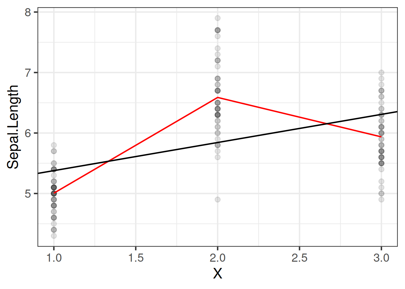
Let’s see what these new models look like:

[R code]
iris_plot2 <-
  iris |>
  mutate(
    predlm2 = predict(iris_lm2)
  ) |>
  arrange(X) |>
  ggplot(aes(x = X, y = Sepal.Length)) +
  geom_point(alpha = .1) +
  geom_line(aes(y = predlm2), col = "red") +
  geom_abline(
    intercept = coef(iris_lm1)[1],
    slope = coef(iris_lm1)[2]
  ) +
  theme_bw(base_size = 18)

print(iris_plot2)
Figure 8

Let’s see how R did that:

[R code]
formula(iris_lm2)
#> Sepal.Length ~ Species
model.matrix(iris_lm2) |>
  as_tibble() |>
  unique()
Table 14

This format is called a “corner point parametrization” (e.g., in Dobson and Barnett (2018)) or “treatment coding” (e.g., in Dunn and Smyth (2018)).

The default contrasts are controlled by options("contrasts"):

[R code]
options("contrasts")
#> $contrasts
#>         unordered           ordered 
#> "contr.treatment"      "contr.poly"

See ?options for more details.

[R code]
formula(iris_lm2_no_int)
#> Sepal.Length ~ Species - 1
model.matrix(iris_lm2_no_int) |>
  as_tibble() |>
  unique()
Table 15

This format is called a “group point parametrization” (e.g., in Dobson and Barnett (2018)).

There are more options; see Dobson and Barnett (2018) §6.4.1 and the codingMatrices package vignette (Venables (2023)).

2.10 Ordinal covariates

(c.f. Dobson and Barnett (2018) §2.4.4)

Example 2 The hers data (Vittinghoff et al. 2012) is available in the rmb package:

[R code]
hers <- rmb::hers |> haven::zap_labels()
[R code]
hers |> head()
Table 16: HERS data

The physact variable records each participant’s self-reported physical activity, relative to other women her age, on an ordered five-level scale (1 = much less active, …, 5 = much more active). We make it an ordered factor so that lm() uses polynomial contrasts, which respect the ordering, instead of the default treatment contrasts:

[R code]
hers <- hers |>
  dplyr::mutate(physact_ord = ordered(physact))

lm_physact <- lm(LDL ~ physact_ord, data = hers)
[R code]
lm_physact |>
  parameters::model_parameters() |>
  parameters::print_md()
Table 17: Mean LDL by physical-activity level, using polynomial contrasts
Parameter Coefficient SE 95% CI t(2747) p
(Intercept) 144.71 0.85 (143.05, 146.38) 170.10 < .001
physact ord (linear) -0.31 2.29 (-4.80, 4.18) -0.14 0.892
physact ord (quadratic) -1.86 2.05 (-5.88, 2.15) -0.91 0.363
physact ord (cubic) 0.47 1.74 (-2.94, 3.89) 0.27 0.785
physact ord (4th degree) -0.58 1.42 (-3.36, 2.21) -0.40 0.686

With polynomial contrasts, each coefficient summarizes a trend component across the ordered levels: the linear term measures the strength and direction of a straight-line (monotone) trend in mean LDL across the levels, and the quadratic and higher terms capture curvature. The contrasts are orthonormal, so the linear coefficient is scaled by the contrast normalization; it is not the raw change in mean LDL per level. Here the linear-trend coefficient is small and not statistically significant, so these data show little evidence of a monotone association between physical-activity level and mean LDL cholesterol.

Working with ordinal variables

When working with ordinal covariates in linear models:

  1. Use ordered() or factor(ordered = TRUE) to create the variable
  2. Consider using polynomial contrasts (contr.poly) which respect ordering
  3. Alternatively, treat the ordinal variable as numeric if equal spacing is reasonable
  4. Check ?codingMatrices::contr.diff for additional contrast options

See Dobson and Barnett (2018) §2.4.4 for more details on contrasts for ordinal variables.

3 Fitting linear models

3.1 Likelihood

\[ \begin{aligned} \mathcal{L}_i &\stackrel{\text{def}}{=}p(Y_i=y_i|\tilde{X}_i = \tilde{x}_i) \\ &= (2\pi\sigma^2)^{-1/2} \operatorname{exp}\mathopen{}\left\{-\frac{1}{2\sigma^2}\varepsilon_i^2\right\}\mathclose{} \\ \varepsilon_i &\stackrel{\text{def}}{=}y_i - \mu_i \\ \mu_i &\stackrel{\text{def}}{=}\mu(x_i) \\ &= x_i \cdot \beta \end{aligned} \]

\[ \begin{aligned} \mathcal{L}&\stackrel{\text{def}}{=}\mathcal{L}(\tilde{y}|\mathbf{x}, \tilde{\beta}, \sigma^2) \\ &\stackrel{\text{def}}{=}\operatorname{p}(\tilde{Y}=\tilde{y}| \mathbf{X}= \mathbf{x}) \\ &= \prod_{i=1}^n \mathcal{L}_i \end{aligned} \tag{5}\]

3.2 Log-likelihood

\[ \begin{aligned} \ell_i &\stackrel{\text{def}}{=}\operatorname{log}\mathopen{}\left\{\mathcal{L}_i\right\}\mathclose{} \\ &= \operatorname{log}\mathopen{}\left\{(2\pi\sigma^2)^{-1/2} \operatorname{exp}\mathopen{}\left\{-\frac{1}{2\sigma^2}\varepsilon_i^2\right\}\mathclose{}\right\}\mathclose{} \\ &= -\frac{1}{2}\operatorname{log}\mathopen{}\left\{2\pi\sigma^2\right\}\mathclose{} -\frac{1}{2\sigma^2}\varepsilon_i^2 \end{aligned} \]

\[ \begin{aligned} \ell &\stackrel{\text{def}}{=}\ell(\tilde{y}|\mathbf{x},\beta, \sigma^2) \\ &\stackrel{\text{def}}{=}\operatorname{log}\mathopen{}\left\{\mathcal{L}(\tilde{y}|\mathbf{x},\beta, \sigma^2)\right\}\mathclose{} \\ &= \operatorname{log}\mathopen{}\left\{\prod_{i=1}^n\mathcal{L}_i\right\}\mathclose{} \\ &= \sum_{i=1}^n\operatorname{log}\mathopen{}\left\{\mathcal{L}_i\right\}\mathclose{} \\ &= \sum_{i=1}^n\ell_i \\ &= \sum_{i=1}^n\mathopen{}\left(-\frac{1}{2}\operatorname{log}\mathopen{}\left\{2\pi\sigma^2\right\}\mathclose{} -\frac{1}{2\sigma^2}\varepsilon_i^2\right)\mathclose{} \\ &= -\frac{n}{2}\operatorname{log}\mathopen{}\left\{2\pi\sigma^2\right\}\mathclose{} - \frac{1}{2\sigma^2}\sum_{i=1}^n \varepsilon_i^2 \\ &= -\frac{n}{2}\operatorname{log}\mathopen{}\left\{2\pi\sigma^2\right\}\mathclose{} - \frac{1}{2\sigma^2}\mathopen{}\left(\tilde{\varepsilon}\cdot \tilde{\varepsilon}\right)\mathclose{} \\ &= -\frac{n}{2}\operatorname{log}\mathopen{}\left\{2\pi\sigma^2\right\}\mathclose{} - \frac{1}{2\sigma^2}\mathopen{}\left((\tilde{y}- \tilde{\mu}) \cdot (\tilde{y}- \tilde{\mu})\right)\mathclose{} \\ &= -\frac{n}{2}\operatorname{log}\mathopen{}\left\{2\pi\sigma^2\right\}\mathclose{} - \frac{1}{2\sigma^2}\mathopen{}\left((\tilde{y}- \mathbf{X}\tilde{\beta}) \cdot (\tilde{y}- \mathbf{X}\tilde{\beta})\right)\mathclose{} \\ &= -\frac{n}{2}\operatorname{log}\mathopen{}\left\{2\pi\sigma^2\right\}\mathclose{} - \frac{1}{2\sigma^2}\sum_{i=1}^n \mathopen{}\left(y_i - \mathopen{}\left(\tilde{x}_i\cdot \tilde{\beta}\right)\mathclose{}\right)\mathclose{}^2 \end{aligned} \tag{6}\]

3.3 Score function

\[ \begin{aligned} \mu_i' &\stackrel{\text{def}}{=}\frac{\partial}{\partial \tilde{\beta}} \mu_i \\ &= \frac{\partial}{\partial \tilde{\beta}} \mathopen{}\left(\tilde{x}_i \cdot \tilde{\beta}\right)\mathclose{} \\ &= \mathopen{}\left( \frac{\partial}{\partial \tilde{\beta}} \tilde{\beta}\right)\mathclose{} \tilde{x}_i \\ &= \mathbb{I}\tilde{x}_i \\ &= \tilde{x}_i \end{aligned} \]

\[ \begin{aligned} \varepsilon'_i &\stackrel{\text{def}}{=}\frac{\partial}{\partial \tilde{\beta}}\varepsilon_i \\ &= \frac{\partial}{\partial \tilde{\beta}} (y_i - \mu_i) \\ &= \frac{\partial}{\partial \tilde{\beta}}y_i - \frac{\partial}{\partial \tilde{\beta}} \mu_i \\ &= 0 - \tilde{x}_i \\ &= - \tilde{x}_i \end{aligned} \]

\[ \begin{aligned} \ell'_i &\stackrel{\text{def}}{=}\frac{\partial}{\partial \tilde{\beta}}\ell_i \\ &= \frac{\partial}{\partial \tilde{\beta}} \mathopen{}\left(-\frac{1}{2}\operatorname{log}\mathopen{}\left\{2\pi\sigma^2\right\}\mathclose{} -\frac{1}{2\sigma^2}\varepsilon_i^2\right)\mathclose{} \\ &= \frac{\partial}{\partial \tilde{\beta}}\mathopen{}\left(-\frac{1}{2}\operatorname{log}\mathopen{}\left\{2\pi\sigma^2\right\}\mathclose{}\right)\mathclose{} - \frac{\partial}{\partial \tilde{\beta}}\frac{1}{2\sigma^2}\varepsilon_i^2 \\ &= 0 - \frac{1}{2\sigma^2}\frac{\partial}{\partial \tilde{\beta}}\varepsilon_i^2 \\ &= - \frac{1}{2\sigma^2}2 \mathopen{}\left(\varepsilon_i'\right)\mathclose{} \varepsilon_i \\ &= - \frac{1}{\sigma^2} \mathopen{}\left(- \tilde{x}_i \varepsilon_i\right)\mathclose{} \\ &= \frac{1}{\sigma^2} \tilde{x}_i \varepsilon_i \end{aligned} \]

\[ \begin{aligned} \ell'_{\tilde{\beta}} &\stackrel{\text{def}}{=}\frac{\partial}{\partial \tilde{\beta}}\ell_{\tilde{\beta}} \\ &= \frac{\partial}{\partial \tilde{\beta}} \sum_{i=1}^n\ell_i \\ &= \sum_{i=1}^n\frac{\partial}{\partial \tilde{\beta}} \ell_i \\ &= \sum_{i=1}^n\ell_i' \\ &= \sum_{i=1}^n\frac{1}{\sigma^2} \tilde{x}_i \varepsilon_i \\ &= \frac{1}{\sigma^2} \sum_{i=1}^n\tilde{x}_i \varepsilon_i \\ &= \frac{1}{\sigma^2} \mathbf{X}^{\top} \tilde{\varepsilon} \end{aligned} \]

3.4 Solving the score equation

To find the MLE, we set the score equal to zero. The score equation for \(\tilde{\beta}\) is:

\[ \ell'_{\tilde{\beta}} = \tilde{0} \]

Since \(\sigma^2 > 0\), this is equivalent to:

\[ \sum_{i=1}^n\tilde{x}_i \varepsilon_i = \tilde{0} \]

Substitute \(\varepsilon_i = y_i - (\tilde{x}_i \cdot \tilde{\beta})\):

\[ \begin{aligned} \tilde{0} &= \sum_{i=1}^n\tilde{x}_i \mathopen{}\left(y_i - (\tilde{x}_i \cdot \tilde{\beta})\right)\mathclose{} \\ &= \sum_{i=1}^n\tilde{x}_i y_i - \sum_{i=1}^n\tilde{x}_i (\tilde{x}_i \cdot \tilde{\beta}) \end{aligned} \]

So the vector score equation is:

\[ \sum_{i=1}^n\tilde{x}_i (\tilde{x}_i \cdot \tilde{\beta}) = \sum_{i=1}^n\tilde{x}_i y_i \]

Assume the design matrix \(\mathbf{X}\) has full column rank. This implies that \(\sum_{i=1}^n \tilde{x}_i {\tilde{x}_i}^{\top}\) is invertible. To solve for \(\tilde{\beta}\), use \(\tilde{x}_i (\tilde{x}_i \cdot \tilde{\beta}) = (\tilde{x}_i {\tilde{x}_i}^{\top})\tilde{\beta}\):

\[ \begin{aligned} \mathopen{}\left(\sum_{i=1}^n\tilde{x}_i {\tilde{x}_i}^{\top}\right)\mathclose{}\tilde{\beta}&= \sum_{i=1}^n\tilde{x}_i y_i \\ \tilde{\beta}&= \mathopen{}\left(\sum_{i=1}^n\tilde{x}_i {\tilde{x}_i}^{\top}\right)\mathclose{}^{-1}\sum_{i=1}^n\tilde{x}_i y_i \\ \hat{\tilde{\beta}}&= ({\mathbf{X}}^{\top}\mathbf{X})^{-1}{\mathbf{X}}^{\top}\tilde{y} \end{aligned} \]

3.5 Hessian

\[ \begin{aligned} \ell_i'' &\stackrel{\text{def}}{=}\frac{\partial}{\partial \tilde{\beta}^{\top}}\frac{\partial}{\partial \tilde{\beta}} \ell_i \\ &= \frac{\partial}{\partial \tilde{\beta}^{\top}} \ell_i' \\ &= \frac{\partial}{\partial \tilde{\beta}^{\top}} \mathopen{}\left(\frac{1}{\sigma^2} \tilde{x}_i \varepsilon_i\right)\mathclose{} \\ &= \frac{1}{\sigma^2} \tilde{x}_i \varepsilon_i'^{\top} \\ &= \frac{1}{\sigma^2} \tilde{x}_i (-\tilde{x}_i^{\top}) \\ &= -\frac{1}{\sigma^2} \tilde{x}_i \tilde{x}_i^{\top} \end{aligned} \]

\[ \begin{aligned} \ell'' &\stackrel{\text{def}}{=}\frac{\partial}{\partial \tilde{\beta}^{\top}}\frac{\partial}{\partial \tilde{\beta}} \ell \\ &= \frac{\partial}{\partial \tilde{\beta}^{\top}} \ell' \\ &= \frac{\partial}{\partial \tilde{\beta}^{\top}} \sum_{i=1}^n\ell_i' \\ &= \sum_{i=1}^n\frac{\partial}{\partial \tilde{\beta}^{\top}} \ell_i' \\ &= \sum_{i=1}^n\ell_i'' \\ &= \sum_{i=1}^n-\frac{1}{\sigma^2} \tilde{x}_i \tilde{x}_i^{\top} \\ &= -\frac{1}{\sigma^2} \sum_{i=1}^n\tilde{x}_i \tilde{x}_i^{\top} \\ &= -\frac{1}{\sigma^2} \mathbf{X}^{\top}\mathbf{X} \end{aligned} \] That is,

\[\ell''= -\frac{1}{\sigma^2} \sum_{i=1}^n\tilde{x}_i \tilde{x}_i^{\top} \tag{7}\]

3.6 Alternative approach using matrix derivatives

\[ \begin{aligned} \ell'_{\tilde{\beta}}(\tilde{y}|\mathbf{x}, \tilde{\beta}, \sigma^2) &\stackrel{\text{def}}{=}\frac{\partial}{\partial \tilde{\beta}}\ell_{\tilde{\beta}}(\tilde{y}|\mathbf{x}, \tilde{\beta}, \sigma^2) \\ &= - \frac{1}{2\sigma^2}\frac{\partial}{\partial \tilde{\beta}} \mathopen{}\left(\sum_{i=1}^n \mathopen{}\left(y_i - \mathopen{}\left(\tilde{x}_i\cdot \tilde{\beta}\right)\mathclose{}\right)\mathclose{}^2\right)\mathclose{} \end{aligned} \tag{8}\]

\[ \sum_{i=1}^n (y_i - \tilde{x}_i^{\top} \tilde{\beta})^2 = (\tilde{y}- \mathbf{X}\tilde{\beta}) \cdot (\tilde{y}- \mathbf{X}\tilde{\beta}) \]

So

\[ \begin{aligned} (\tilde{y}- \mathbf{X}\tilde{\beta})'(\tilde{y}- \mathbf{X}\tilde{\beta}) &= (\tilde{y}' - \tilde{\beta}'X')(\tilde{y}- \mathbf{X}\tilde{\beta}) \\ &= \tilde{y}'\tilde{y}- \tilde{\beta}'X'\tilde{y}- \tilde{y}'\mathbf{X}\tilde{\beta}+\tilde{\beta}'\mathbf{X}'\mathbf{X}\beta \\ &= \tilde{y}'\tilde{y}- 2\tilde{y}'\mathbf{X}\beta +\beta'\mathbf{X}'\mathbf{X}\beta \end{aligned} \]

\[ \begin{aligned} \frac{\partial}{\partial \tilde{\beta}}\mathopen{}\left(\sum_{i=1}^n (y_i - x_i' \beta)^2\right)\mathclose{} &= \frac{\partial}{\partial \tilde{\beta}}(\tilde{y}- X\beta)'(\tilde{y}- X\beta) \\ &= \frac{\partial}{\partial \tilde{\beta}} (y'y - 2y'X\beta +\beta'\mathbf{X}'\mathbf{X}\beta) \\ &= (- 2X'y +2\mathbf{X}'\mathbf{X}\beta) \\ &= - 2X'(y - X\beta) \\ &= - 2X'(y - \operatorname{E}[y]) \\ &= - 2X' \varepsilon(y) \end{aligned} \tag{9}\]

So if \(\ell'(\beta,\sigma^2) = 0\), then

\[ \begin{aligned} 0 &= (- 2X'y +2\mathbf{X}'\mathbf{X}\beta)\\ 2X'y &= 2\mathbf{X}'\mathbf{X}\beta\\ X'y &= \mathbf{X}'\mathbf{X}\beta\\ (\mathbf{X}'\mathbf{X})^{-1}X'y &= \beta \end{aligned} \]

Hessian

The Hessian (second derivative matrix) is:

\[ \begin{aligned} \ell_{\beta, \beta'} ''(\beta, \sigma^2;\tilde{y}, \mathbf{X}) &= -\frac{1}{2\sigma^2}\mathbf{X}'\mathbf{X} \end{aligned} \]

\(\ell_{\beta, \beta'} ''(\beta, \sigma^2;\mathbf X,\tilde{y})\) is negative definite at \(\beta = (\mathbf{X}'\mathbf{X})^{-1}X'y\), so \(\hat \beta_{ML} = (\mathbf{X}'\mathbf{X})^{-1}X'y\) is the MLE for \(\beta\).

Similarly (not shown):

\[ \hat\sigma^2_{ML} = \frac{1}{n} (Y-X\hat\beta)'(Y-X\hat\beta) \]

3.7 Residual Standard Deviation

[R code]
sigma(bw_lm2)
#> [1] 180.613

\(\sigma\) is NOT “Residual standard error”

[R code]
summary(bw_lm2)
#> 
#> Call:
#> lm(formula = weight ~ sex + age + sex:age, data = bw)
#> 
#> Residuals:
#>    Min     1Q Median     3Q    Max 
#> -246.7 -138.1  -39.1  176.6  274.3 
#> 
#> Coefficients:
#>             Estimate Std. Error t value Pr(>|t|)    
#> (Intercept)  -2141.7     1163.6   -1.84  0.08057 .  
#> sexmale        873.0     1611.3    0.54  0.59395    
#> age            130.4       30.0    4.35  0.00031 ***
#> sexmale:age    -18.4       41.8   -0.44  0.66389    
#> ---
#> Signif. codes:  0 '***' 0.001 '**' 0.01 '*' 0.05 '.' 0.1 ' ' 1
#> 
#> Residual standard error: 181 on 20 degrees of freedom
#> Multiple R-squared:  0.643,  Adjusted R-squared:  0.59 
#> F-statistic:   12 on 3 and 20 DF,  p-value: 0.000101

3.8 Predicted and fitted values

Definition 3 (Predicted value) In a regression model \(\operatorname{p}(y|\tilde{x})\), the predicted value of \(y\) given \(\tilde{x}\) is the estimated mean of \(Y\) given \(\tilde{X}=\tilde{x}\):

\[\hat y \stackrel{\text{def}}{=}\mathop{\hat{\operatorname{E}}}\nolimits\mathopen{}\left[Y|\tilde{X}=\tilde{x}\right]\mathclose{}\]

For linear models, the predicted value can be straightforwardly calculated by multiplying each predictor value \(x_j\) by its corresponding coefficient \(\beta_j\) and adding up the results:

\[ \begin{aligned} \hat y &= \mathop{\hat{\operatorname{E}}}\nolimits\mathopen{}\left[Y|\tilde{X}=\tilde{x}\right]\mathclose{} \\ &= {\tilde{x}}^{\top}\hat\beta \\ &= \hat\beta_0\cdot 1 + \hat\beta_1 x_1 + ... + \hat\beta_p x_p \end{aligned} \]

Definition 4 (Fitted value) For a given dataset \((\tilde{Y}, \mathbf{X})\) and corresponding fitted model \(\operatorname{p}_{\hat \beta}(\tilde{y}|\mathbf{x})\), the fitted value of \(y_i\) is the predicted value (see Definition 3) of \(y\) when \(\tilde{X}=\tilde{x}_i\) using the estimated parameters \(\hat \beta\):

\[\hat y_i \stackrel{\text{def}}{=}\mathop{\hat{\operatorname{E}}}\nolimits\mathopen{}\left[Y_i|\tilde{X}=\tilde{x}_i\right]\mathclose{} = {\tilde{x}_i}^{\top}\hat \beta\]

Example: prediction for the birthweight data

[R code]
x <- c(1, 1, 40)
sum(x * coef(bw_lm1))
#> [1] 3225.49

R has built-in functions for prediction:

[R code]
x <- tibble(age = 40, sex = "male")
bw_lm1 |> predict(newdata = x)
#>       1 
#> 3225.49

If you don’t provide newdata, R will use the covariate values from the original dataset:

[R code]
predict(bw_lm1)
#>       1       2       3       4       5       6       7       8       9      10 
#> 3225.49 3062.45 2983.70 2578.87 3225.49 3062.45 2621.02 2820.66 2741.91 3304.24 
#>      11      12      13      14      15      16      17      18      19      20 
#> 2862.81 2941.56 3346.38 3062.45 3225.49 2699.77 2862.81 2578.87 2983.70 2820.66 
#>      21      22      23      24 
#> 3225.49 2941.56 2983.70 3062.45

These special predictions are called the fitted values of the dataset (see Definition 4).

R has an extra function to get these values:

[R code]
fitted(bw_lm1)
#>       1       2       3       4       5       6       7       8       9      10 
#> 3225.49 3062.45 2983.70 2578.87 3225.49 3062.45 2621.02 2820.66 2741.91 3304.24 
#>      11      12      13      14      15      16      17      18      19      20 
#> 2862.81 2941.56 3346.38 3062.45 3225.49 2699.77 2862.81 2578.87 2983.70 2820.66 
#>      21      22      23      24 
#> 3225.49 2941.56 2983.70 3062.45

4 Assessing model fit

4.1 Goodness of fit

AIC and BIC

When we use likelihood ratio tests, we are comparing how well different models fit the data.

Likelihood ratio tests require nested models: one must be a special case of the other.

AIC and BIC can be used to compare both nested and non-nested models.

Formulas

Definition 5 (Akaike Information Criterion (AIC)) \[\text{AIC} = -2 \ell(\hat\theta) + 2 p\]

where \(\ell(\hat\theta)\) is the log-likelihood evaluated at the maximum-likelihood estimates \(\hat\theta\), \(p\) is the number of estimated parameters (including \(\hat\sigma^2\) for Gaussian models), and \(n\) is the number of observations.

Definition 6 (Bayesian Information Criterion (BIC)) \[\text{BIC} = -2 \ell(\hat\theta) + p \log(n)\]

where \(\ell(\hat\theta)\), \(p\), and \(n\) are defined as in Definition 5.

Conceptual basis

Each criterion has two components:

  • Fit term (\(-2\ell(\hat\theta)\)): measures lack of fit — lower is better. A model with more parameters will always achieve a higher (or equal) log-likelihood on the observed data.

  • Penalty term (\(2 p\) for AIC; \(p \log(n)\) for BIC): penalizes model complexity to guard against overfitting.

Together, they balance goodness of fit against parsimony.

AIC vs. BIC

Criterion Penalty per parameter Tends to select
AIC \(2\) larger models
BIC \(\log(n)\) smaller models

The BIC penalty exceeds the AIC penalty whenever \(\log(n) > 2\), i.e., when \(n > e^2 \approx 7.4\). In practice, BIC almost always penalizes additional parameters more heavily than AIC and therefore tends to select simpler (more parsimonious) models (Vittinghoff et al. 2012; Kleinbaum et al. 2014).

AIC in R

[R code]
-2 * logLik(bw_lm2) |> as.numeric() +
  2 * (length(coef(bw_lm2)) + 1) # sigma counts as a parameter here
#> [1] 323.159

AIC(bw_lm2)
#> [1] 323.159

BIC in R

[R code]
-2 * logLik(bw_lm2) |> as.numeric() +
  (length(coef(bw_lm2)) + 1) * log(nobs(bw_lm2))
#> [1] 329.049

BIC(bw_lm2)
#> [1] 329.049

Interpretation

  • Lower values are better. There are no hypothesis tests or p-values associated with these criteria.

  • To compare models, calculate the criterion for each model and choose the model with the smallest value.

  • Differences of less than 2 units are generally considered negligible; differences greater than 10 are considered strong evidence in favor of the lower-criterion model.

  • BIC tends to favor simpler models than AIC, especially when the sample size is large.

(Residual) Deviance

Let \(q\) be the number of distinct covariate combinations in a data set.

[R code]
bw_X_unique <-
  bw |>
  count(sex, age)

n_unique_bw <- nrow(bw_X_unique)

For example, in the birthweight data, there are \(q = 12\) unique patterns (Table 18).

[R code]
bw_X_unique
Table 18: Unique covariate combinations in the birthweight data, with replicate counts

Definition 7 (Replicates) If a given covariate pattern has more than one observation in a dataset, those observations are called replicates.

Example 3 (Replicates in the birthweight data) In the birthweight dataset, there are 2 replicates of the combination “female, age 36” (Table 18).

Exercise 14 (Replicates in the birthweight data) Which covariate pattern(s) in the birthweight data has the most replicates?

Solution 1 (Replicates in the birthweight data). Two covariate patterns are tied for most replicates: males at age 40 weeks and females at age 40 weeks. 40 weeks is the usual length for human pregnancy (Polin et al. (2011)), so this result makes sense.

[R code]
bw_X_unique |> dplyr::filter(n == max(n))

Saturated models

The most complicated model we could fit would have one parameter (a mean) for each covariate pattern, plus a variance parameter:

[R code]
lm_max <-
  bw |>
  mutate(age = factor(age)) |>
  lm(
    formula = weight ~ sex:age - 1,
    data = _
  )

lm_max |>
  parameters() |>
  print_md()
Table 19: Saturated model for the birthweight data
Parameter Coefficient SE 95% CI t(12) p
sex (male) × age35 2925.00 187.92 (2515.55, 3334.45) 15.56 < .001
sex (female) × age36 2570.50 132.88 (2280.98, 2860.02) 19.34 < .001
sex (male) × age36 2625.00 187.92 (2215.55, 3034.45) 13.97 < .001
sex (female) × age37 2539.00 187.92 (2129.55, 2948.45) 13.51 < .001
sex (male) × age37 2737.50 132.88 (2447.98, 3027.02) 20.60 < .001
sex (female) × age38 2872.50 132.88 (2582.98, 3162.02) 21.62 < .001
sex (male) × age38 2982.00 108.50 (2745.60, 3218.40) 27.48 < .001
sex (female) × age39 2846.00 132.88 (2556.48, 3135.52) 21.42 < .001
sex (female) × age40 3152.25 93.96 (2947.52, 3356.98) 33.55 < .001
sex (male) × age40 3256.25 93.96 (3051.52, 3460.98) 34.66 < .001
sex (male) × age41 3292.00 187.92 (2882.55, 3701.45) 17.52 < .001
sex (female) × age42 3210.00 187.92 (2800.55, 3619.45) 17.08 < .001

We call this model the full, maximal, or saturated model for this dataset.

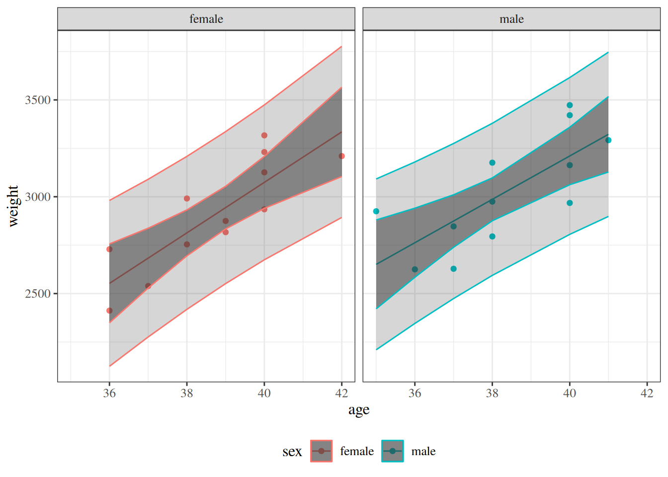
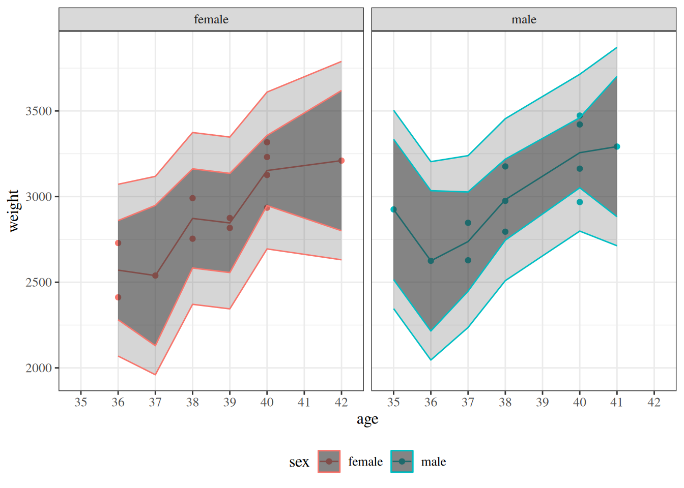
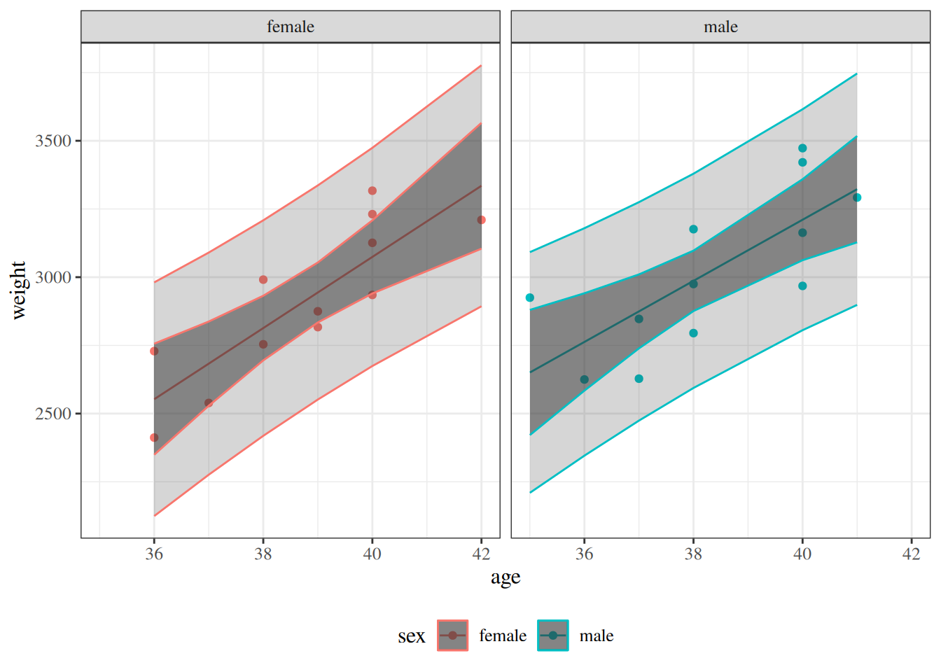
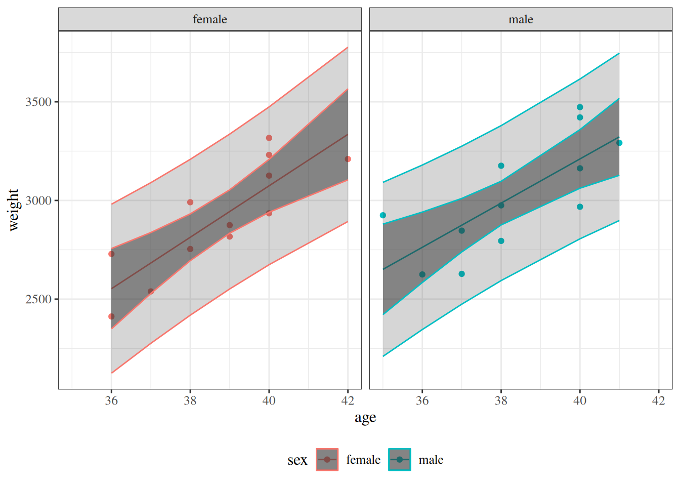
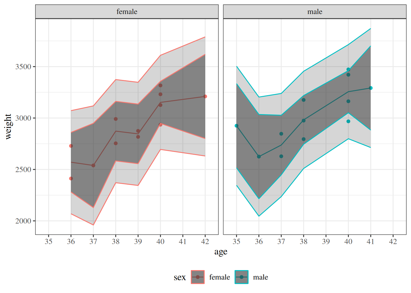
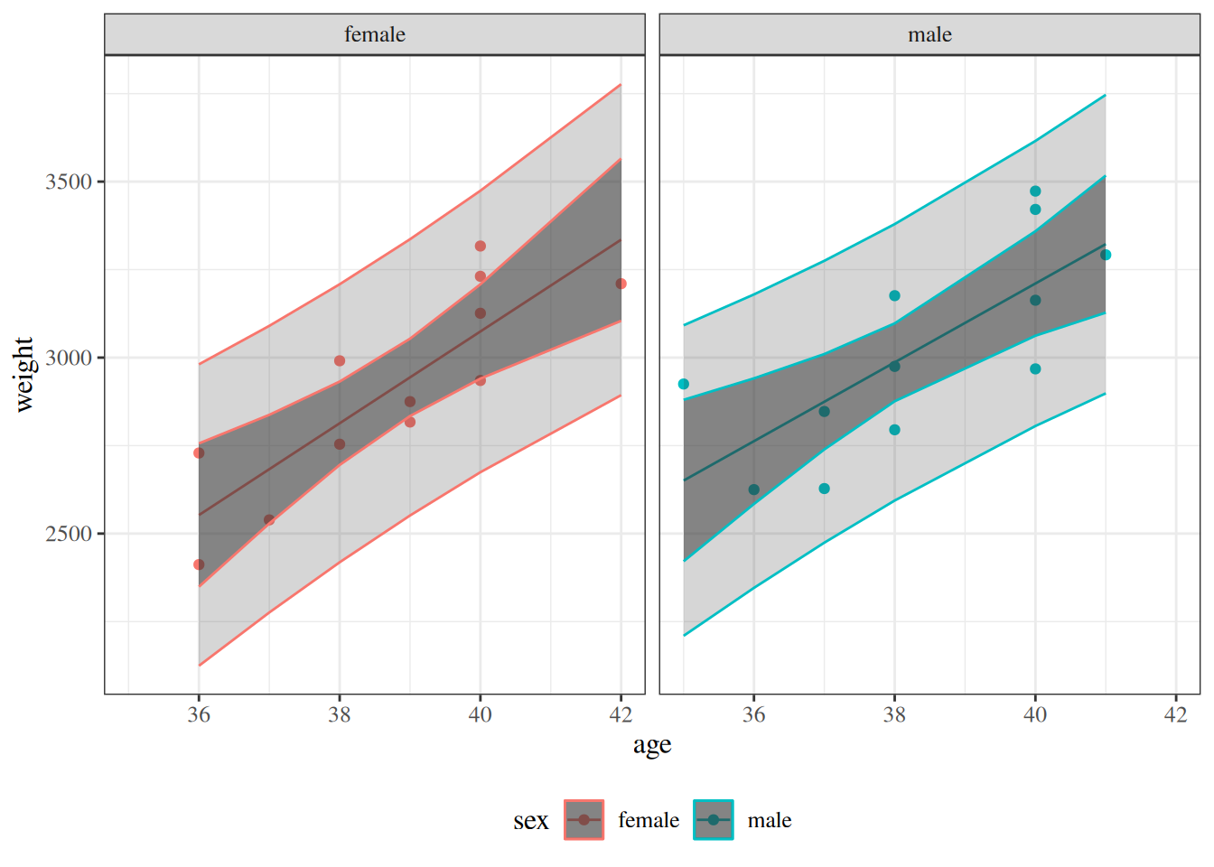
Figure 9: Model 2 and saturated model for birthweight data, with confidence and prediction intervals
[R code]
plot_PIs_and_CIs(bw, bw_lm2)
(a) Model 2 (linear with age:sex interaction)

[R code]
plot_PIs_and_CIs(bw |> mutate(age = factor(age)), lm_max)
(b) Saturated model

We can calculate the log-likelihood of this model as usual:

[R code]
logLik(lm_max)
#> 'log Lik.' -151.402 (df=13)

We can compare this model to our other models using chi-square tests, as usual:

[R code]
library(lmtest)
lrtest(lm_max, bw_lm2)

The likelihood ratio statistic for this test is \[\lambda = 2 * (\ell_{\text{full}} - \ell) = 10.355374\] where:

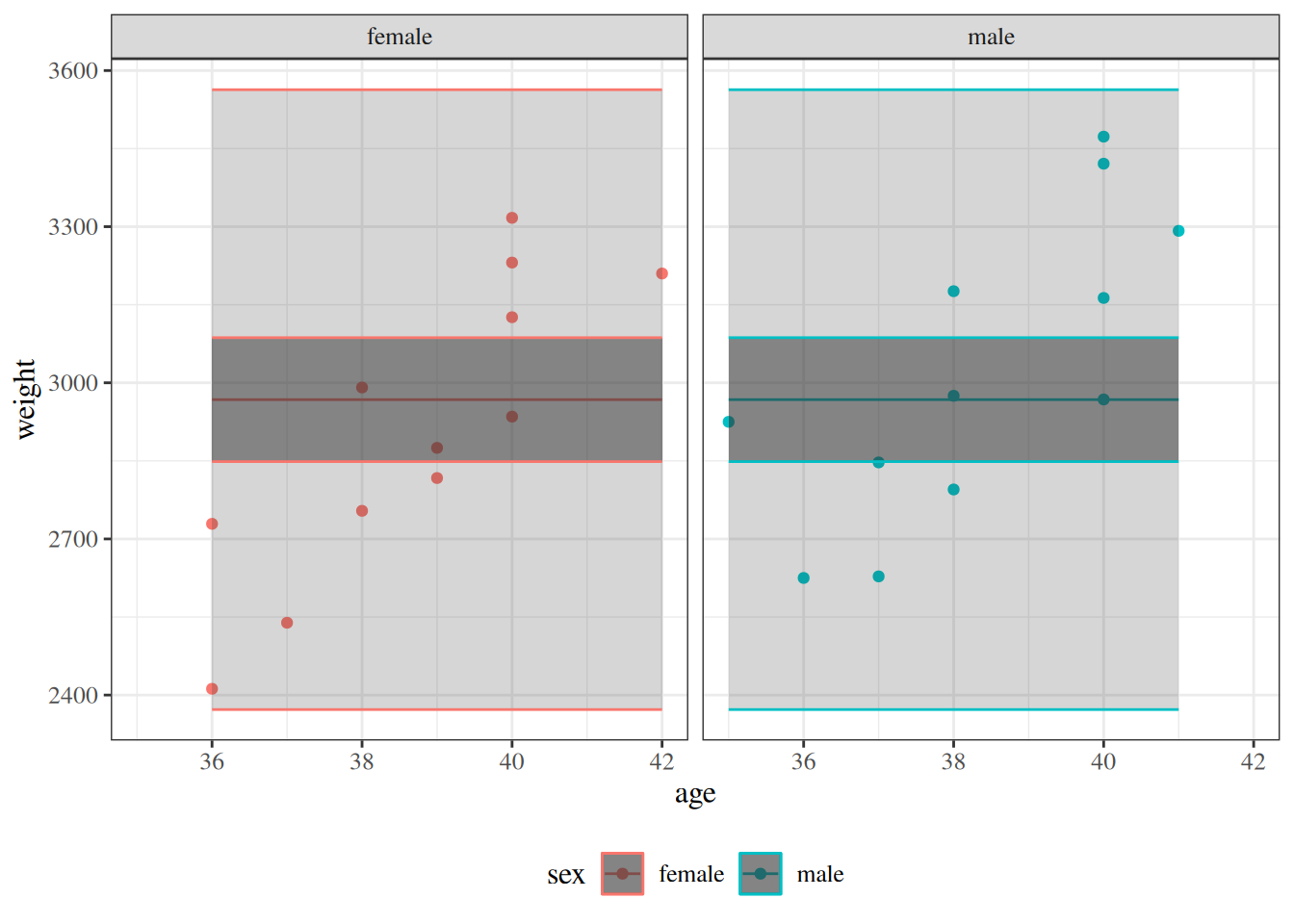
  • \(\ell_{\text{full}}\) is the log-likelihood of the full model: -151.401601
  • \(\ell\) is the log-likelihood of our comparison model (two slopes, two intercepts): -156.579288

This statistic is called the deviance or residual deviance for our two-slopes and two-intercepts model; it tells us how much the likelihood of that model deviates from the likelihood of the maximal model.

The corresponding p-value tells us whether there we have enough evidence to detect that our two-slopes, two-intercepts model is a worse fit for the data than the maximal model; in other words, it tells us if there’s evidence that we missed any important patterns. (Remember, a nonsignificant p-value could mean that we didn’t miss anything and a more complicated model is unnecessary, or it could mean we just don’t have enough data to tell the difference between these models.)

Null Deviance

Similarly, the least complicated model we could fit would have only one mean parameter, an intercept:

\[\operatorname{E}\mathopen{}\left[Y|X=x\right]\mathclose{} = \beta_0\]

We can fit this model in R like so:

[R code]
lm0 <- lm(weight ~ 1, data = bw)

lm0 |>
  parameters() |>
  print_md()
Parameter Coefficient SE 95% CI t(23) p
(Intercept) 2967.67 57.58 (2848.56, 3086.77) 51.54 < .001
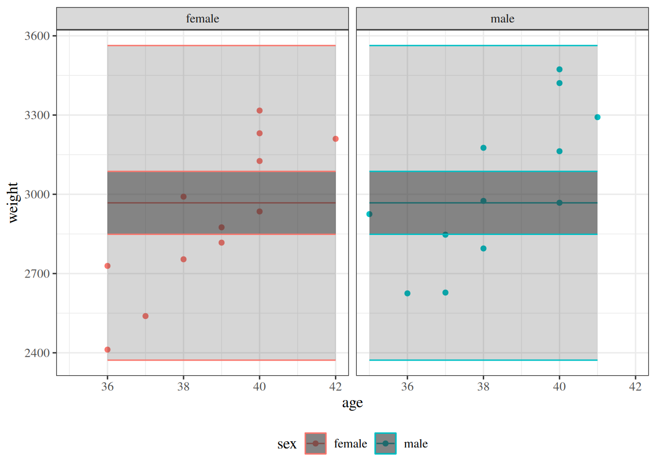
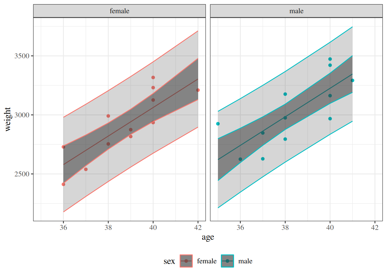
Figure 10: Null model and model 2 for birthweight data, with 95% confidence and prediction intervals.
[R code]
plot_PIs_and_CIs(bw, lm0)
(a) Null model

[R code]
plot_PIs_and_CIs(bw, bw_lm2)
(b) Model 2 (linear with age:sex interaction)

This model also has a likelihood:

[R code]
logLik(lm0)
#> 'log Lik.' -168.955 (df=2)

And we can compare it to more complicated models using a likelihood ratio test:

[R code]
lrtest(bw_lm2, lm0)

The likelihood ratio statistic for the test comparing the null model to the maximal model is \[\lambda = 2 * (\ell_{\text{full}} - \ell_{0}) = 35.106732\] where:

  • \(\ell_{\text{0}}\) is the log-likelihood of the null model: -168.954967
  • \(\ell_{\text{full}}\) is the log-likelihood of the maximal model: -151.401601

In R, this test is:

[R code]
lrtest(lm_max, lm0)

This log-likelihood ratio statistic is called the null deviance. It tells us whether we have enough data to detect a difference between the null and full models.

Figure 11: Four models for birthweight data, with 95% confidence and prediction intervals. The spectrum from null to saturated includes many other possible models, such as quadratic polynomial models (with or without interactions) and generalized additive models (GAMs).
[R code]
plot_PIs_and_CIs(bw, lm0)
(a) Null model

[R code]
plot_PIs_and_CIs(bw, bw_lm1)
(b) No-interactions model (parallel slopes)

[R code]
plot_PIs_and_CIs(bw, bw_lm2)
(c) Model 2 (linear with age:sex interaction)

[R code]
plot_PIs_and_CIs(bw |> mutate(age = factor(age)), lm_max)
(d) Saturated model

Gaussian Deviance vs. GLM Deviance

The residual deviance is a general concept that applies to all GLMs, including Gaussian linear regression. For any GLM, the residual deviance is:

\[D = 2(\ell_{\text{sat}} - \ell(\hat\beta)) \tag{10}\]

where \(\ell_{\text{sat}}\) is the log-likelihood of the saturated model and \(\ell(\hat\beta)\) is the log-likelihood of the fitted model. However, this formula simplifies differently depending on the distribution family, and the resulting test statistics have different null distributions.

Gaussian linear regression deviance

From Equation 6, the Gaussian log-likelihood is:

\[ \ell(\hat\beta, \hat\sigma^2) = -\frac{n}{2}\log(2\pi\hat\sigma^2) - \frac{1}{2\hat\sigma^2} \sum_{i=1}^n(y_i - \hat{y}_i)^2 \]

The saturated model has one free mean parameter per distinct covariate pattern. When there are no replicates (each covariate pattern appears exactly once), it sets \(\hat\mu_i = y_i\) for every observation, so its residual sum of squares is zero:

\[\ell_{\text{sat}}(\hat\sigma^2) = -\frac{n}{2}\log(2\pi\hat\sigma^2)\]

Substituting into Equation 10, the Gaussian deviance simplifies to the residual sum of squares (RSS), scaled by \(\hat\sigma^2\):

\[ D = 2(\ell_{\text{sat}} - \ell(\hat\beta)) = \frac{\sum_{i=1}^n(y_i - \hat{y}_i)^2}{\hat\sigma^2} = \frac{\text{RSS}}{\hat\sigma^2} \]

Because \(\sigma^2\) is unknown and must be estimated, comparing deviances between two nested Gaussian models uses an F-test, which is exact under Gaussian assumptions. Substituting \(D = \text{RSS}/\hat\sigma^2\), the \(\hat\sigma^2\) factors cancel:

\[ F = \frac{(D_1 - D_2) / (p_2 - p_1)}{D_2 / (n - p_2)} = \frac{(\text{RSS}_1 - \text{RSS}_2) / (p_2 - p_1)}{\text{RSS}_2 / (n - p_2)} \ \sim \ F_{p_2 - p_1,\; n - p_2} \]

In R, deviance() applied to an lm object returns RSS (the unscaled deviance):

deviance(bw_lm2)
#> [1] 652425
sum(residuals(bw_lm2)^2)
#> [1] 652425

The Gaussian linear regression model can equivalently be fit as a GLM with family = gaussian, which also returns RSS as the deviance:

bw_glm2 <- glm(
  weight ~ sex + age + sex:age,
  data = bw,
  family = gaussian
)

deviance(bw_lm2)
#> [1] 652425
deviance(bw_glm2)
#> [1] 652425

Non-Gaussian GLM deviance

For non-Gaussian GLMs, the deviance does not simplify to RSS. The formula depends on the distribution family:

Poisson:

\[ D = 2\sum_{i=1}^n \left[y_i \log\!\left(\frac{y_i}{\hat\mu_i}\right) - (y_i - \hat\mu_i)\right] \]

Binomial:

\[ D = 2\sum_{i=1}^n \left[y_i \log\!\left(\frac{y_i}{\hat\pi_i}\right) + (n_i - y_i)\log\!\left(\frac{n_i - y_i}{n_i - \hat\pi_i}\right)\right] \]

For Poisson and Binomial models, the dispersion parameter \(\phi = 1\) is fixed rather than estimated. Consequently, the difference in deviances between two nested models follows an approximate \(\chi^2\) distribution:

\[D_1 - D_2 \;\dot \sim\; \chi^2_{p_2 - p_1}\]

This asymptotic result replaces the exact F-test used for Gaussian models.

Saturated vs. fully parametrized models with replicates

When some covariate patterns appear more than once (i.e., when there are replicates), it is important to distinguish between two special models:

  • The saturated model has one free mean parameter per distinct covariate pattern (\(q\) parameters, where \(q \leq n\) is the number of unique patterns).
  • The fully parametrized model has one free mean parameter per observation (\(n\) parameters).

When there are no replicates (\(q = n\)), these two coincide. When there are replicates (\(q < n\)), the saturated model constrains all observations sharing a covariate pattern to have the same mean, but places no constraint on means across different patterns. See Kleinbaum and Klein (2010) for further discussion of this distinction.

Deviance is always measured relative to the saturated model, not the fully parametrized model.

Gaussian deviance with replicates

When covariate pattern \(k\) has \(n_k\) replicates with sample mean \(\bar{y}_k\), the saturated model fits \(\hat\mu_k = \bar{y}_k\) for each pattern \(k\), so its residual sum of squares equals the within-group (pure error) SS:

\[ \text{RSS}_{\text{sat}} = \sum_{k=1}^q \sum_{i: \tilde{x}_i = \tilde{x}_k} (y_i - \bar{y}_k)^2 \]

This is nonzero whenever any covariate pattern has replicates with different response values. The Gaussian deviance relative to the saturated model is therefore:

\[ D = 2(\ell_{\text{sat}} - \ell(\hat\beta)) = \frac{\text{RSS} - \text{RSS}_{\text{sat}}}{\hat\sigma^2} \]

Note

R’s deviance() applied to an lm object returns the total fitted-model RSS, not the deviance relative to the saturated model. To compute the deviance relative to the saturated model, subtract the saturated model’s RSS: deviance(lm_fit) - deviance(lm_saturated).

For the birthweight data, we can verify this directly using bw_lm2 (the interaction model) and lm_max (the saturated model):

deviance(bw_lm2)                      # total RSS of fitted model
#> [1] 652425
deviance(lm_max)                      # within-group (pure error) SS
#> [1] 423783
deviance(bw_lm2) - deviance(lm_max)   # lack-of-fit SS (deviance vs. saturated)
#> [1] 228642
GLM deviance with replicates

For a Binomial GLM fit to data grouped by covariate pattern (with \(y_k\) events and \(n_k\) observations for pattern \(k\)), the saturated model sets \(\hat\pi_k^{\text{sat}} = y_k / n_k\) for each pattern \(k\). R’s deviance() correctly computes \(2(\ell_{\text{sat}} - \ell(\hat\beta))\) using this grouping:

\[ D = 2\sum_{k=1}^q \left[ y_k \log\!\left(\frac{y_k / n_k}{\hat\pi_k}\right) + (n_k - y_k)\log\!\left(\frac{1 - y_k/n_k}{1 - \hat\pi_k}\right) \right] \]

When binomial data is ungrouped (individual Bernoulli observations, \(n_i = 1\)), R uses the fully parametrized model as its reference — assigning \(\hat\pi_i = y_i \in \{0, 1\}\) to each individual observation. Since each predicted probability is exactly 0 or 1, every Bernoulli likelihood contribution equals 1, and hence \(\ell_{\text{fp}} = 0\). Thus R’s deviance() returns \(-2\ell(\hat\beta)\).

We can verify this directly: observations are ungrouped Bernoulli with repeated covariate patterns (\(x \in \{0, 1\}\) appears three times each).

set.seed(42)
x_ug <- rep(0:1, each = 3)
y_ug <- c(0L, 1L, 0L, 1L, 1L, 0L)
fit_ug <- glm(y_ug ~ x_ug, family = binomial)
deviance(fit_ug)                     # R's deviance
#> [1] 7.63817
-2 * as.numeric(logLik(fit_ug))      # -2 * log-likelihood (using ell_fp = 0)
#> [1] 7.63817

Note

This reference model is the fully parametrized model (one parameter per observation), not the saturated model (one parameter per distinct covariate pattern). They coincide only when there are no repeated covariate patterns (\(q = n\)). When patterns do repeat (\(q < n\)), the saturated model sets \(\hat\pi_k = y_k/n_k\) per pattern, giving \(\ell_{\text{sat}} < 0\).

deviance() for ungrouped data cannot be used as a goodness-of-fit test against the \(\chi^2\) distribution when \(q < n\). The correct GOF statistic is \(2(\ell_{\text{sat}} - \ell(\hat\beta))\), but R’s deviance() for ungrouped data returns \(-2\ell(\hat\beta)\) (using \(\ell_{\text{fp}} = 0\)). These two quantities differ by \(-2\ell_{\text{sat}} > 0\) whenever \(q < n\). Even if each covariate pattern has many replicates (large \(n_k\)), R’s ungrouped deviance is the wrong statistic to compare against \(\chi^2(q - p)\). To obtain a valid GOF test when patterns repeat, fit the model using grouped data (one row per pattern with \(y_k\) and \(n_k\)), so that R uses the saturated model as its reference.

For further discussion, see Dunn and Smyth (2018, chap. 9) and this Stats Stack Exchange thread.

Summary

Feature Gaussian linear regression Non-Gaussian GLMs (e.g., Poisson, Binomial)
Deviance formula \((\text{RSS} - \text{RSS}_{\text{sat}})/\hat\sigma^2\) \(2(\ell_{\text{sat}} - \ell(\hat\beta))\)
deviance() in R Returns total RSS Returns \(2(\ell_{\text{sat}} - \ell(\hat\beta))\)
Saturated model reference Per covariate pattern Per covariate pattern (grouped) or per observation (ungrouped)
Dispersion \(\phi\) Unknown; estimated as \(s^2 = \text{RSS}/(n-p)\) Fixed (\(\phi = 1\))
Test for nested models F-test (exact) \(\chi^2\)-test (asymptotic)

4.2 Diagnostics

Tip

This section is adapted from Dobson and Barnett (2018, secs. 6.2–6.3) and Dunn and Smyth (2018) Chapter 3.

Assumptions in linear regression models

\[Y_i|\tilde{X}_i \sim_{{\color{red}{\perp\!\!\!\perp}}} {\color{blue}{\operatorname{N}}}({\color{orange}{\mu_i}}, {\color{green}{\sigma^2}})\] \[{\color{orange}{\mu_i = \tilde{x}\cdot \tilde{\beta}}}\]

  1. Normality

The model assumes that the distribution conditional on a given \(X\) value is Gaussian.

  1. Correct Functional Form of Conditional Mean Structure (Linear Component)

The model assumes that the conditional means have the structure: \[\operatorname{E}\mathopen{}\left[Y|\tilde{X}= \tilde{x}\right]\mathclose{} = {\tilde{x}}^{\top}\tilde{\beta}\]

  1. Homoskedasticity

The model assumes that variance \(\sigma^2\) is constant (with respect to \(\tilde{x}\)).

  1. Independence

Direct visualization

[R code]
bw <-
  bw |>
  mutate(
    predlm2 = predict(bw_lm2)
  ) |>
  arrange(sex, age)

plot1_interact <-
  plot1 %+% bw +
  geom_line(aes(y = predlm2))

print(plot1_interact)
Figure 12: Birthweight model with interaction term

Fitted model for hers data

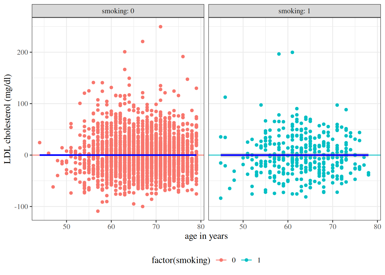
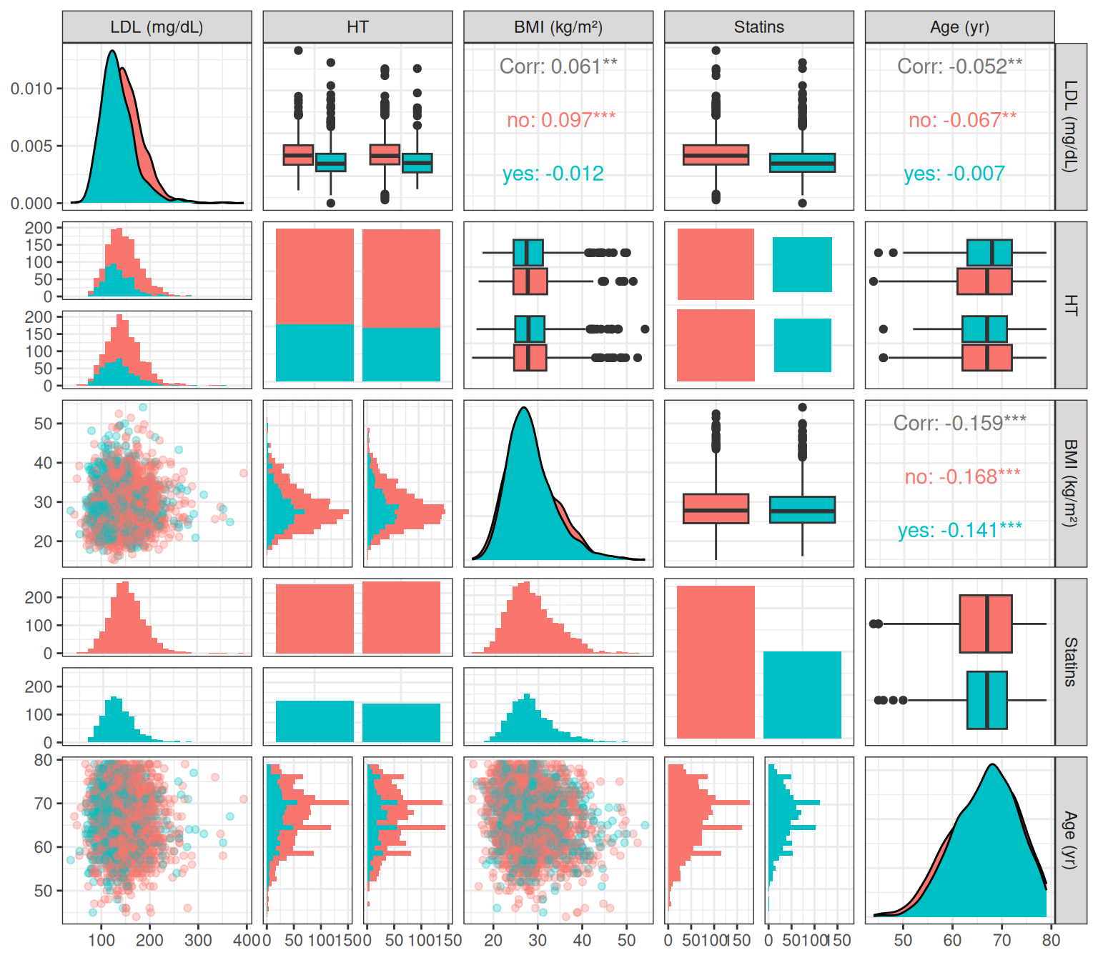
Consider the hers data from Vittinghoff et al. (2012).

The “heart and estrogen/progestin study” (HERS) was a clinical trial of hormone therapy for prevention of recurrent heart attacks and death among 2,763 post-menopausal women with existing coronary heart disease (CHD) (Hulley et al. 1998).

The trial was conducted at 20 US clinical centers. Participants were randomized to receive either conjugated equine estrogens (0.625 mg/day) plus medroxyprogesterone acetate (2.5 mg/day) or a matching placebo (Hulley et al. 1998). Women were followed for an average of 4.1 years (Hulley et al. 1998).

The primary outcome was nonfatal myocardial infarction or CHD death (Hulley et al. 1998).

[R code]
hers <- rmb::hers |> haven::zap_labels()
hers
Table 20: hers data
[R code]
hers_lm_with_int <- lm(
  na.action = na.exclude,
  LDL ~ smoking * age, data = hers
)


library(equatiomatic)
equatiomatic::extract_eq(hers_lm_with_int)

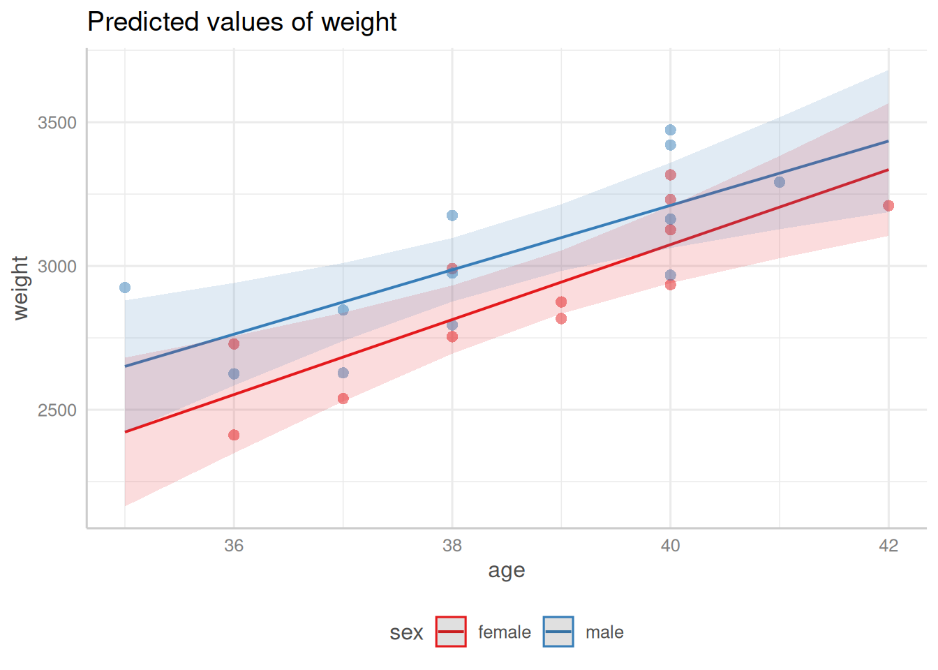
\[ \operatorname{LDL} = \alpha + \beta_{1}(\operatorname{smoking}) + \beta_{2}(\operatorname{age}) + \beta_{3}(\operatorname{smoking} \times \operatorname{age}) + \epsilon \]

[R code]
hers_lm_no_int <- lm(
  na.action = na.exclude,
  LDL ~ age + smoking:age - 1, data = hers
)

library(equatiomatic)
equatiomatic::extract_eq(hers_lm_no_int)

\[ \operatorname{LDL} = \beta_{1}(\operatorname{age}) + \beta_{2}(\operatorname{age} \times \operatorname{age}_{\operatorname{smoking}}) + \epsilon \]

Table 21: hers data models with and without intercepts
[R code]
library(gtsummary)
hers_lm_with_int |> 
  tbl_regression(intercept = TRUE)
(a) With intercept
Characteristic Beta 95% CI p-value
(Intercept) 154 138, 170 <0.001
current smoker 54 15, 94 0.007
age in years -0.14 -0.38, 0.09 0.2
current smoker * age in years -0.79 -1.4, -0.17 0.012
Abbreviation: CI = Confidence Interval
[R code]
hers_lm_no_int |> 
  tbl_regression(intercept = TRUE)
(b) No intercept
Characteristic Beta 95% CI p-value
age in years 2.1 2.1, 2.2 <0.001
age in years * current smoker 0.19 0.12, 0.26 <0.001
Abbreviation: CI = Confidence Interval
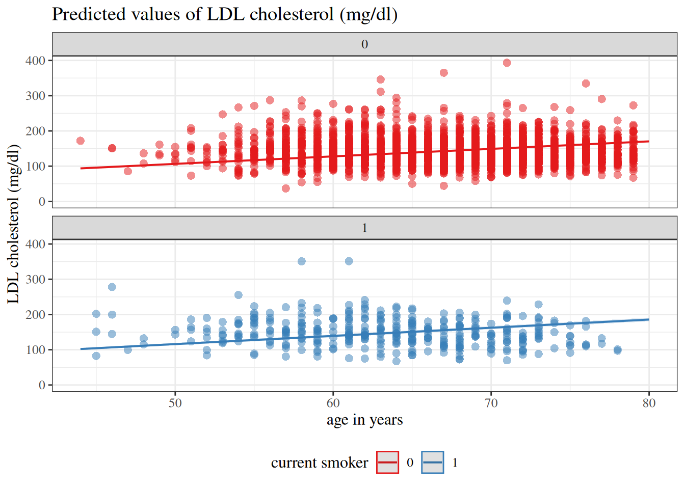
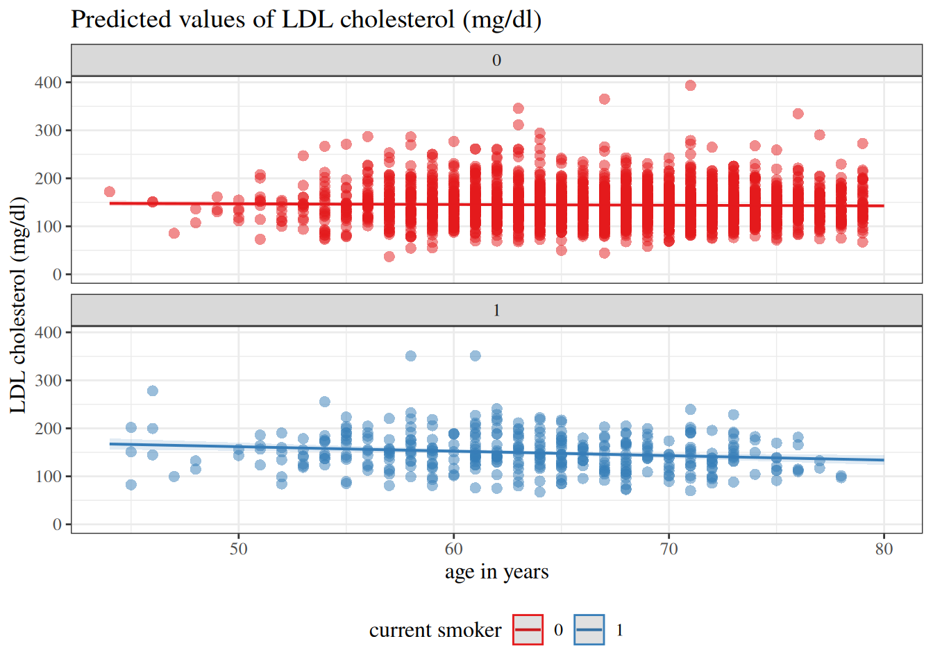
Figure 13: hers data models with and without intercepts
[R code]
library(sjPlot)

hers_plot1 <- hers_lm_no_int |>
  sjPlot::plot_model(
    type = "pred",
    terms = c("age", "smoking"),
    show.data = TRUE
  ) +
  facet_wrap(~group_col, ncol = 1) +
  expand_limits(y = 0) +
  theme(legend.position = "bottom")

hers_plot1
(a) No intercept

[R code]
library(sjPlot)

hers_plot2 <- hers_lm_with_int |>
  sjPlot::plot_model(
    type = "pred",
    terms = c("age", "smoking"),
    show.data = TRUE
  ) +
  facet_wrap(~group_col, ncol = 1) +
  expand_limits(y = 0) +
  theme(legend.position = "bottom")

hers_plot2
(b) With intercept

Residuals

Definition 8 (Deviation of an observation from its subpopulation mean) The deviation of an observation from its subpopulation mean in a probabilistic model \(p(Y \mid X)\), is the difference between an observed value and its model-implied mean given covariates:

\[e(y_i) \stackrel{\text{def}}{=}y_i - \operatorname{E}\mathopen{}\left[Y_i \mid X_i\right]\mathclose{} \tag{11}\]

We can rearrange Equation 11 to view \(y_i\) as the sum of its mean plus the deviation (often called error/noise):

\[y_i = \operatorname{E}\mathopen{}\left[Y_i \mid X_i\right]\mathclose{} + e(y_i)\]

Definition 9 (Signal (statistical sense)) In statistical modeling, the signal is the deterministic part of the model. For mean-based models, the signal is the model-implied mean function, for example \(\operatorname{E}\mathopen{}\left[Y \mid X\right]\mathclose{}\) (or \(\operatorname{E}\mathopen{}\left[Y\right]\mathclose{}\) when there are no covariates).

Theorem 1 (Deviations in Gaussian models) If \(Y\) has a Gaussian distribution, then \(e(Y)\) also has a Gaussian distribution, and vice versa.

Proof. By Definition 8, \(e(Y \mid X = x) = Y - \operatorname{E}\mathopen{}\left[Y \mid X = x\right]\mathclose{}\). Let \(\mu(x) = \operatorname{E}\mathopen{}\left[Y \mid X = x\right]\mathclose{}\). Since \(e(Y \mid X = x) = Y - \mu(x)\) is an affine function of \(Y\), and Gaussian distributions are closed under affine transformations, if \(Y \mid X = x \sim \operatorname{N}(\mu(x), \sigma^2)\), then:

\[ e(Y \mid X = x) = Y - \mu(x) \sim \operatorname{N}(\mu(x) - \mu(x), \sigma^2) = \operatorname{N}(0, \sigma^2) \]

Conversely, since \(Y = \operatorname{E}\mathopen{}\left[Y \mid X = x\right]\mathclose{} + e(Y \mid X = x) = \mu(x) + e(Y \mid X = x)\), if \(e(Y \mid X = x) \sim \operatorname{N}(0, \sigma^2)\), then \(Y \mid X = x = \mu(x) + e(Y \mid X = x) \sim \operatorname{N}(\mu(x), \sigma^2)\).

Definition 10 (Residuals) A residual is the difference between an observed value and its corresponding fitted value, \(\hat y\): \[ \begin{aligned} r&\stackrel{\text{def}}{=}y - \hat y \end{aligned} \]

For indexed observations, this is equivalently: \[ r_i \stackrel{\text{def}}{=}y_i - \hat y_i \]

For a particular fitted model, each residual \(r_i\) is tied to its corresponding fitted value \(\hat y_i\). The fitted value \(\hat y_i\) is often a sample mean or fitted conditional mean, but not always.

Example 4 (Residuals in birthweight data)  

[R code]
plot1_interact +
  facet_wrap(~sex) +
  geom_segment(
    aes(
      x = age,
      y = predlm2,
      xend = age,
      yend = weight,
      col = sex,
      group = id
    ),
    linetype = "dotted"
  )
Figure 14: Fitted values and residuals for interaction model for birthweight data

4.3 Residuals of fitted values vs subpopulation-mean deviations

The residual is a plug-in estimate of the deviation of an observation from its subpopulation mean:

\[ \begin{aligned} e(y_i) &= y_i - \operatorname{E}\mathopen{}\left[Y_i \mid X_i\right]\mathclose{} \\ \widehat{e(y_i)} &= y_i - \hat y_i \\ &= r_i \end{aligned} \]

Different sources are not fully consistent about these terms. For terminology in this course, we use:

  • deviation for deviation of an observation from its population mean (typically conditional on covariates). This quantity is often called error in other sources, even though it doesn’t directly involve an estimate; cf., https://en.wikipedia.org/wiki/Errors_and_residuals;
  • estimation error for deviation of an estimate from its estimand;
  • residual for deviation of an observed value from a fitted value.

4.4 General characteristics of residuals

Definition 11 (Hat matrix) For an ordinary least squares linear model with design matrix \(\mathbf{X}\), the hat matrix is

\[H = \mathbf{X}({\mathbf{X}}^{\top}\mathbf{X})^{-1}{\mathbf{X}}^{\top}\]

so the fitted values satisfy

\[\hat{\tilde{Y}} = H\tilde{Y}\]

Theorem 2 (Mean and variance of residuals) For an ordinary least squares linear model with fitted values \(\hat y_i = \tilde{x}_i \cdot \tilde{\beta}\) (and fitted-value vector \(\hat{\tilde{Y}}\)), if the conditional mean is correctly specified so that:

\[ \operatorname{E}\mathopen{}\left[\tilde{Y}\mid \mathbf{X}\right]\mathclose{} = \mathbf{X}\beta\]

equivalently:

\[ \operatorname{E}\mathopen{}\left[\hat{\tilde{Y}} \mid \mathbf{X}\right]\mathclose{} = \operatorname{E}\mathopen{}\left[\tilde{Y}\mid \mathbf{X}\right]\mathclose{}\]

and if the errors are homoskedastic so that \(\operatorname{Var}\mathopen{}\left(\tilde{Y}\mid \mathbf{X}\right)\mathclose{} = \sigma^2\mathbb{I}_n\) where \(\mathbb{I}_n\) is the \(n \times n\) identity matrix, then, treating \(\mathbf{X}\) as fixed in this derivation, the residual moments are:

\[\operatorname{E}\mathopen{}\left[\tilde{r} \mid \mathbf{X}\right]\mathclose{} = 0 \tag{12}\] \[\operatorname{Var}\mathopen{}\left(r_i \mid \mathbf{X}\right)\mathclose{} = \sigma^2(1-h_{ii}) \tag{13}\]

The conditional mean result (Equation 12) uses unbiasedness of fitted values. The conditional variance result (Equation 13) uses the homoskedasticity condition with the OLS hat-matrix representation.

When leverage is roughly uniform, \(h_{ii} \approx k/n\), where \(k = \mathrm{rank}(\mathbf{X})\) (so \(k = p + 1\) for a full-rank model with an intercept and \(p\) predictors), so \(\operatorname{Var}\mathopen{}\left(r_i\right)\mathclose{} \approx \sigma^2\) as \(n\) grows.

Proof. Equation 12:

\[ \begin{aligned} \operatorname{E}\mathopen{}\left[{\tilde{r}} \mid \mathbf{X}\right]\mathclose{} &= \operatorname{E}\mathopen{}\left[\tilde{Y}- \hat{\tilde{Y}} \mid \mathbf{X}\right]\mathclose{} \\ &= \operatorname{E}\mathopen{}\left[\tilde{Y}\mid \mathbf{X}\right]\mathclose{} - \operatorname{E}\mathopen{}\left[\hat{\tilde{Y}} \mid \mathbf{X}\right]\mathclose{} \\ &= \operatorname{E}\mathopen{}\left[\tilde{Y}\mid \mathbf{X}\right]\mathclose{} - \operatorname{E}\mathopen{}\left[H\tilde{Y}\mid \mathbf{X}\right]\mathclose{} \\ &= \operatorname{E}\mathopen{}\left[\tilde{Y}\mid \mathbf{X}\right]\mathclose{} - H\operatorname{E}\mathopen{}\left[\tilde{Y}\mid \mathbf{X}\right]\mathclose{} \\ &= \operatorname{E}\mathopen{}\left[\tilde{Y}\mid \mathbf{X}\right]\mathclose{} - H\mathbf{X}\beta \\ &= \mathbf{X}\beta- H\mathbf{X}\beta \\ &= \mathbf{X}\beta- \mathbf{X}\beta \\ &= \tilde{0} \end{aligned} \]

Equation 13:

\[ \begin{aligned} {\tilde{r}} &= (\mathbb{I}_n-H)\tilde{Y} \\ \operatorname{Var}\mathopen{}\left({\tilde{r}} \mid \mathbf{X}\right)\mathclose{} &= \operatorname{Var}\mathopen{}\left((\mathbb{I}_n-H)\tilde{Y}\mid \mathbf{X}\right)\mathclose{} \\ &= (\mathbb{I}_n-H)\operatorname{Var}\mathopen{}\left(\tilde{Y}\mid \mathbf{X}\right)\mathclose{}{(\mathbb{I}_n-H)}^{\top} \\ &= (\mathbb{I}_n-H)\sigma^2\mathbb{I}_n{(\mathbb{I}_n-H)}^{\top} \\ &= \sigma^2(\mathbb{I}_n-H){(\mathbb{I}_n-H)}^{\top} \\ &= \sigma^2(\mathbb{I}_n-H)^2 \\ &= \sigma^2(\mathbb{I}_n - 2H + H^2) \\ &= \sigma^2(\mathbb{I}_n-H) \qquad (\text{since } H^2 = H) \\ \operatorname{Var}\mathopen{}\left(r_i \mid \mathbf{X}\right)\mathclose{} &= \left[\operatorname{Var}\mathopen{}\left({\tilde{r}} \mid \mathbf{X}\right)\mathclose{}\right]_{ii} \\ &= \left[\sigma^2(\mathbb{I}_n-H)\right]_{ii} \\ &= \sigma^2(1-h_{ii}) \end{aligned} \]

Theorem 3 (Conditional distribution of residuals in Gaussian models) In a Gaussian linear regression model, the residuals \(r_i\), conditional on the design matrix \(\mathbf{X}\), are normally distributed:

\[r_i \mid \mathbf{X}\sim \operatorname{N}\mathopen{}\left(0,\; \sigma^2(1 - h_{ii})\right)\mathclose{} \tag{14}\]

where \(h_{ii}\) is the \(i\)-th diagonal element of the hat matrix (Definition 11). When leverage is roughly uniform, \(\sigma^2(1-h_{ii}) \approx \sigma^2\) for large \(n\); replacing the unknown \(\sigma^2\) with its estimate \(\hat \sigma^2\) gives:

\[r_i \approx \operatorname{N}(0, \hat \sigma^2) \tag{15}\]

Proof. Using the hat matrix (Definition 11), the residual vector is \(\tilde{r} = (I-H)\tilde{Y}\), so the \(i\)-th residual is a linear combination of the observations:

\[r_i = [(I-H)\tilde{Y}]_i = \sum_{j=1}^n (\delta_{ij} - h_{ij})\, Y_j\]

where \(\delta_{ij}\) is the Kronecker delta (\(\delta_{ij} = 1\) if \(i = j\), else \(\delta_{ij} = 0\)).

Given \(\mathbf{X}\), the random variables \(Y_1, \ldots, Y_n\) are conditionally independent Gaussians by the Gaussian model assumption. Therefore, conditional on \(\mathbf{X}\), the residual \(r_i\) is a linear combination of independent Gaussians, so \(r_i\) is Gaussian.

The mean and variance follow from Theorem 2:

\[ \begin{aligned} \operatorname{E}\mathopen{}\left[r_i \mid \mathbf{X}\right]\mathclose{} &= 0 \\ \operatorname{Var}\mathopen{}\left(r_i \mid \mathbf{X}\right)\mathclose{} &= \sigma^2(1 - h_{ii}) \end{aligned} \]

Therefore \(r_i \mid \mathbf{X}\sim \operatorname{N}(0, \sigma^2(1 - h_{ii}))\).

4.5 Computing residuals in R

R provides a function for residuals:

[R code]
resid(bw_lm2)
#>         1         2         3         4         5         6         7         8 
#>  176.2667 -140.7333 -144.1333  -59.5333  177.4667 -126.9333  -68.9333  242.6667 
#>         9        10        11        12        13        14        15        16 
#> -139.3333   51.6667  156.6667 -125.1333  274.2759 -137.7069  -27.6897 -246.6897 
#>        17        18        19        20        21        22        23        24 
#> -191.6724  189.3276  -11.6724 -242.6379  -47.6379  262.3621  210.3621  -30.6207

Exercise 15 Check R’s output by computing the residuals directly.

Solution.

[R code]
bw$weight - fitted(bw_lm2)
#>         1         2         3         4         5         6         7         8 
#>  176.2667 -140.7333 -144.1333  -59.5333  177.4667 -126.9333  -68.9333  242.6667 
#>         9        10        11        12        13        14        15        16 
#> -139.3333   51.6667  156.6667 -125.1333  274.2759 -137.7069  -27.6897 -246.6897 
#>        17        18        19        20        21        22        23        24 
#> -191.6724  189.3276  -11.6724 -242.6379  -47.6379  262.3621  210.3621  -30.6207

This matches R’s output!

4.6 Graphing the residuals

Figure 15: Fitted values and residuals for interaction model for birthweight data
[R code]
plot1_interact +
  facet_wrap(~sex) +
  geom_segment(
    aes(
      x = age,
      y = predlm2,
      xend = age,
      yend = weight,
      col = sex,
      group = id
    ),
    linetype = "dotted"
  )
(a) fitted values

[R code]

bw <- bw |>
  mutate(
    resids_intxn =
      weight - fitted(bw_lm2)
  )

plot_bw_resid <-
  bw |>
  ggplot(aes(
    x = age,
    y = resids_intxn,
    linetype = sex,
    shape = sex,
    col = sex
  )) +
  theme_bw() +
  xlab("Gestational age (weeks)") +
  ylab("residuals (grams)") +
  theme(legend.position = "bottom") +
  geom_hline(aes(
    yintercept = 0,
    col = sex
  )) +
  geom_segment(
    aes(yend = 0),
    linetype = "dotted"
  ) +
  geom_point(alpha = .7)
# expand_limits(y = 0, x = 0)
print(plot_bw_resid + facet_wrap(~sex))
(b) Residuals

4.7 Residuals versus predictors

[R code]
hers <- hers |>
  mutate(
    resids_no_intcpt =
      LDL - fitted(hers_lm_no_int),
    resids_with_intcpt =
      LDL - fitted(hers_lm_with_int)
  )
Figure 16: Residuals of hers data vs predictors
[R code]
hers |>
  arrange(age) |>
  ggplot() +
  aes(x = age, y = resids_no_intcpt, col = factor(smoking)) +
  geom_point() +
  geom_hline(aes(yintercept = 0, col = factor(smoking))) +
  facet_wrap(~smoking, labeller = "label_both") +
  theme(legend.position = "bottom") +
  geom_smooth(col = "blue")
(a) no intercept

[R code]
hers |>
  arrange(age) |>
  ggplot() +
  aes(x = age, y = resids_with_intcpt, col = factor(smoking)) +
  geom_point() +
  geom_hline(aes(yintercept = 0, col = factor(smoking))) +
  facet_wrap(~smoking, labeller = "label_both") +
  theme(legend.position = "bottom") +
  geom_smooth(col = "blue")
(b) with intercept

4.8 Residuals versus fitted values

[R code]
library(ggfortify)
hers_lm_no_int |>
  update(na.action = na.omit) |>
  autoplot(
    which = 1,
    ncol = 1,
    smooth.colour = NA
  ) +
  geom_hline(yintercept = 0, col = "red")
Figure 17: Residuals of interaction model for hers data

We can add a LOESS smooth to visualize where the residual mean is nonzero:

[R code]
library(ggfortify)
hers_lm_no_int |>
  update(na.action = na.omit) |>
  autoplot(
    which = 1,
    ncol = 1
  ) +
  geom_hline(yintercept = 0, col = "red")
Figure 18: Residuals of interaction model for hers data, no intercept term
Figure 19: Residuals of interaction model for hers data, with and without intercept term
[R code]
library(ggfortify)
hers_lm_no_int |>
  update(na.action = na.omit) |>
  autoplot(
    which = 1,
    ncol = 1
  ) +
  geom_hline(yintercept = 0, col = "red")
(a) no intercept term

[R code]
hers_lm_with_int |>
  update(na.action = na.omit) |>
  autoplot(
    which = 1,
    ncol = 1
  ) +
  geom_hline(yintercept = 0, col = "red")
(b) with intercept term

Definition 12 (Standardized residuals) For an ordinary linear model, the estimated standard deviation of the \(i\)th residual is

\[ \mathop{\widehat{\operatorname{SD}}}\nolimits\mathopen{}\left(r_i\right)\mathclose{} = \hat{\sigma}\sqrt{1-h_{ii}} \]

so the standardized residual is

\[ r'_i = \frac{r_i}{\mathop{\widehat{\operatorname{SD}}}\nolimits\mathopen{}\left(r_i\right)\mathclose{}} = \frac{r_i}{\hat{\sigma}\sqrt{1-h_{ii}}} \]

Hence, with enough data and a correct model, each standardized residual has an approximately standard Gaussian marginal distribution; that is,

\[ r'_i \ \dot{\sim} \ N(0,1) \]

but they are not independent. If \(H\) is the hat matrix with entries \(h_{ij}\), then

\[ \operatorname{Cov}\mathopen{}\left(r_i,r_j \mid \mathbf{X}\right)\mathclose{} = \begin{cases} \sigma^2(1-h_{ii}), & i=j,\\ -\sigma^2h_{ij}, & i\neq j, \end{cases} \]

and therefore

\[ \operatorname{Cov}\mathopen{}\left(r'_i,r'_j \mid \mathbf{X}\right)\mathclose{} \approx \begin{cases} 1, & i=j,\\ \dfrac{-h_{ij}}{\sqrt{(1-h_{ii})(1-h_{jj})}}, & i\neq j, \end{cases} \]

In particular, for \(i \neq j\), these covariances are generally nonzero.

Marginal distributions of residuals

To look for problems with our model, we can check whether the residuals \(r_i\) and standardized residuals \(r'_i\) look like they have the distributions that they are supposed to have, according to the model.

Standardized residuals in R

[R code]
h_ii <- hatvalues(bw_lm2)
manual_std_resid <- resid(bw_lm2) / (sigma(bw_lm2) * sqrt(1 - h_ii))
manual_std_resid
#>          1          2          3          4          5          6          7 
#>  1.1598166 -0.9260109 -0.8747917 -0.3472255  1.0350665 -0.7347315 -0.3990086 
#>          8          9         10         11         12         13         14 
#>  1.4375164 -0.8253872  0.3060646  0.9280669 -0.8761592  1.9142780 -0.8655921 
#>         15         16         17         18         19         20         21 
#> -0.1642993 -1.4637574 -1.1101599  1.0965787 -0.0676062 -1.4615865 -0.2869582 
#>         22         23         24 
#>  1.5803994  1.2671652 -0.1980543
rstandard(bw_lm2)
#>          1          2          3          4          5          6          7 
#>  1.1598166 -0.9260109 -0.8747917 -0.3472255  1.0350665 -0.7347315 -0.3990086 
#>          8          9         10         11         12         13         14 
#>  1.4375164 -0.8253872  0.3060646  0.9280669 -0.8761592  1.9142780 -0.8655921 
#>         15         16         17         18         19         20         21 
#> -0.1642993 -1.4637574 -1.1101599  1.0965787 -0.0676062 -1.4615865 -0.2869582 
#>         22         23         24 
#>  1.5803994  1.2671652 -0.1980543
[R code]
rstandard_compare_plot <-
  tibble(
    x = resid(bw_lm2) / (sigma(bw_lm2) * sqrt(1 - h_ii)),
    y = rstandard(bw_lm2)
  ) |>
  ggplot(aes(x = x, y = y)) +
  geom_point() +
  theme_bw() +
  coord_equal() +
  xlab("resid(bw_lm2)/(sigma(bw_lm2)*sqrt(1-h_ii))") +
  ylab("rstandard(bw_lm2)") +
  geom_abline(
    aes(
      intercept = 0,
      slope = 1,
      col = "x=y"
    )
  ) +
  labs(colour = "") +
  scale_colour_manual(values = "red")

print(rstandard_compare_plot)

Let’s add these residuals to the tibble of our dataset:

[R code]
bw <-
  bw |>
  mutate(
    fitted_lm2 = fitted(bw_lm2),
    resid_lm2 = resid(bw_lm2),
    resid_lm2_alt = weight - fitted_lm2,
    std_resid_lm2 = rstandard(bw_lm2),
    std_resid_lm2_alt =
      resid_lm2 / (sigma(bw_lm2) * sqrt(1 - h_ii))
  )

bw |>
  select(
    sex,
    age,
    weight,
    fitted_lm2,
    resid_lm2,
    std_resid_lm2
  )
[R code]
resid_marginal_hist <-
  bw |>
  ggplot(aes(x = resid_lm2)) +
  geom_histogram()

print(resid_marginal_hist)
Figure 20: Marginal distribution of (nonstandardized) residuals
[R code]
std_resid_marginal_hist <-
  bw |>
  ggplot(aes(x = std_resid_lm2)) +
  geom_histogram()

print(std_resid_marginal_hist)
Figure 21: Marginal distribution of standardized residuals

QQ plot of standardized residuals

[R code]
library(ggfortify)
# needed to make ggplot2::autoplot() work for `lm` objects

qqplot_lm2_auto <-
  bw_lm2 |>
  autoplot(
    which = 2, # options are 1:6; can do multiple at once
    ncol = 1
  ) +
  theme_classic()

print(qqplot_lm2_auto)

QQ plot: typical patterns

[R code]
set.seed(36) # seed chosen for Fig. 3.6 reproduction
n <- 150     # sample size as in @dunn2018generalized Fig. 3.6

sims <- list(
  "Right skewed"    = rchisq(n, df = 3),
  "Left skewed"     = -rchisq(n, df = 3),
  "Tails too heavy" = rt(n, df = 3),
  "Tails too light" = runif(n, -sqrt(3), sqrt(3)),
  "True normal"     = rnorm(n),
  "Bimodal"         = c(rnorm(n / 2, -2.5), rnorm(n / 2, 2.5))
)

old_par <- par(
  mfcol = c(2, 6),
  mar = c(3, 3, 2, 0.5),
  oma = c(0, 0, 0, 0)
)

for (nm in names(sims)) {
  qqnorm(
    sims[[nm]],
    main = nm,
    xlab = "Theoretical Quantiles",
    ylab = "Sample Quantiles",
    pch = 1,
    cex = 0.6
  )
  qqline(sims[[nm]])
  hist(
    sims[[nm]],
    main = "",
    xlab = "Residuals",
    ylab = "Frequency",
    col = "grey70",
    border = "white",
    breaks = 15
  )
}
[R code]

par(old_par)
Figure 22: Typical QQ-plot patterns for six types of residual distribution. Adapted from Dunn and Smyth (2018, fig. 3.6), with thanks to the authors; reproduced here using simulated data (\(n = 150\)). Each column shows one distribution scenario: a QQ plot (top) paired with a histogram of the simulated data (bottom).

QQ plot - how it’s built

[R code]
bw <- bw |>
  mutate(
    # plotting position: (rank - 0.5) / n
    p = (rank(std_resid_lm2) - 1 / 2) / n(),
    expected_quantiles_lm2 = qnorm(p)
  )

qqplot_lm2 <-
  bw |>
  ggplot(
    aes(
      x = expected_quantiles_lm2,
      y = std_resid_lm2,
      col = sex,
      shape = sex
    )
  ) +
  geom_point() +
  theme_classic() +
  theme(legend.position = "none") + # removing the plot legend
  ggtitle("Normal Q-Q") +
  xlab("Theoretical Quantiles") +
  ylab("Standardized residuals")

# find the reference line through the (theoretical, empirical) quantile pairs
# at probabilities 0.25 and 0.75:

ps <- c(.25, .75) # reference probabilities
a <- quantile(rstandard(bw_lm2), ps) # empirical quantiles
b <- qnorm(ps) # theoretical quantiles

qq_slope <- diff(a) / diff(b)
qq_intcpt <- a[1] - b[1] * qq_slope

qqplot_lm2 <-
  qqplot_lm2 +
  geom_abline(slope = qq_slope, intercept = qq_intcpt)
Figure 23: Three equivalent ways to produce a QQ plot of the standardized residuals for the birthweight model (Equation 2). All three plots show the same data and reference line.
[R code]
print(qqplot_lm2)
(a) ggplot2 (manual construction)

[R code]
std_resid_lm2 <- rstandard(bw_lm2)

qqnorm(
  std_resid_lm2,
  main = "Normal Q-Q",
  xlab = "Theoretical Quantiles",
  ylab = "Standardized residuals"
)
qqline(std_resid_lm2)
(b) base R (qqnorm + qqline)

[R code]
library(ggfortify)
autoplot(
  bw_lm2,
  which = 2,
  ncol = 1
) +
  theme_classic()
(c) ggfortify::autoplot()

Formal diagnostic tests for linear regression assumptions

Graphical diagnostics are usually the first step, but formal tests can provide numerical summaries.

For linear regression residuals, three common tests are:

  • fligner.test() for equal variances across groups (the Fligner–Killeen test).
  • Levene / Brown–Forsythe test (a median-centered Levene variant, where standard Levene centers on group means, and Brown–Forsythe centers on group medians for more robustness; e.g., via car::leveneTest(..., center = median) or equivalent code).
  • shapiro.test() / Shapiro–Wilk test for normality.

Fligner–Killeen test (homoskedasticity across groups)

Suppose residuals are split into groups (\(g = 1, \ldots, G\)), for example by a categorical predictor.

The test starts from absolute deviations from each group median: \[ d_{gi} = |e_{gi} - \text{median}(e_{g1}, \ldots, e_{g,n_g})|. \]

After ranking the pooled \(d_{gi}\) values, the Fligner–Killeen statistic is built from normal scores of those ranks.

Under the null hypothesis of equal variances, the test statistic is approximately \(\chi^2_{G-1}\). Small p-values suggest heteroskedasticity.

Levene / Brown–Forsythe test (homoskedasticity across groups)

Levene’s test transforms residuals to within-group absolute deviations: \[ z_{gi} = |e_{gi} - c_g|, \] where \(c_g\) is the group center.

Classical Levene uses the group mean for \(c_g\). Brown–Forsythe uses the group median, which is more robust.

Then run a one-way ANOVA on \(z_{gi}\) by group: \[ F = \frac{\text{MS}_{\text{between}}}{\text{MS}_{\text{within}}} \sim F_{G-1, N-G} \quad\text{under }H_0. \]

Small p-values suggest unequal residual variance.

For simple linear regression, Kutner et al. (2005, 116–17) describes the Brown–Forsythe test by splitting observations into two \(X\)-level groups (low versus high), computing absolute deviations from each group median, and applying a two-sample pooled-variance t test: let \[ z_{ij} = |e_{ij} - \tilde e_i|, \] where \(j\) indexes observations within group \(i\), and \(\tilde e_i\) is the median residual in group \(i\). Then: \[ t_{\text{BF}} = \frac{\bar z_{1} - \bar z_{2}} {s_p \sqrt{1/n_{1} + 1/n_{2}}}, \quad t_{\text{BF}} \approx t_{n_{1}+n_{2}-2} \text{ under }H_0. \] Here, \(\bar z_{1}\) and \(\bar z_{2}\) are the means of the \(z_{ij}\) values in groups \(i=1\) and \(i=2\), \(s_p\) is their pooled standard deviation, and \(n_{1}, n_{2}\) are the two group sample sizes. Large \(|t_{\text{BF}}|\) indicates nonconstant residual variance.

Shapiro–Wilk test (normality of standardized residuals)

For ordered standardized residuals \(r_{(1)} \le \cdots \le r_{(n)}\), the Shapiro–Wilk statistic is: \[ W = \frac{\left(\sum_{i=1}^n a_i r_{(i)}\right)^2} {\sum_{i=1}^n (r_i - \bar r)^2}, \] where \(a_i\) are constants from normal-order-statistic moments. The numerator uses ordered residuals \(r_{(i)}\), while the denominator uses the original (unordered) residuals.

If residuals are Gaussian, \(W\) tends to be close to 1. Small \(W\) (and small p-value) indicates departure from normality.

Numerical example (birthweight interaction model)

[R code]
diag_bw <-
  broom::augment(bw_lm2, data = bw) |>
  transmute(
    sex,
    resid_lm2 = .resid,
    std_resid_lm2 = .std.resid
  )

fligner_bw <- fligner.test(resid_lm2 ~ sex, data = diag_bw)

levene_bw <-
  diag_bw |>
  group_by(sex) |>
  mutate(
    med_resid = median(resid_lm2),
    abs_dev = abs(resid_lm2 - med_resid)
  ) |>
  ungroup()

levene_fit <- aov(abs_dev ~ sex, data = levene_bw)
levene_tab <- summary(levene_fit)[[1]]
levene_F <- unname(levene_tab[1, "F value"])
levene_p <- unname(levene_tab[1, "Pr(>F)"])

shapiro_bw <- shapiro.test(diag_bw$std_resid_lm2)

tibble(
  test = c(
    "Fligner--Killeen: equal variance by sex",
    "Levene/Brown--Forsythe: equal variance by sex",
    "Shapiro--Wilk: normality of standardized residuals"
  ),
  statistic = c(
    unname(fligner_bw$statistic),
    levene_F,
    unname(shapiro_bw$statistic)
  ),
  p_value = c(
    fligner_bw$p.value,
    levene_p,
    shapiro_bw$p.value
  )
) |>
  mutate(
    statistic = signif(statistic, 4),
    p_value = signif(p_value, 4)
  )

Interpretation rule: for all three tests, a small p-value is evidence against the corresponding model assumption.

Compared with visual diagnostics:

  • Fligner–Killeen / Levene summarizes the same heteroskedasticity signal that we inspect in residuals-vs-fitted (Figure 24) and scale-location (Figure 32) plots.
  • Shapiro–Wilk summarizes the same normality signal that we inspect in QQ plots (Figure 23 (c)) and standardized-residual histograms (Figure 21).
  • Use tests and plots together: the tests provide a single numerical summary, while the plots show the shape and practical size of departures.

Conditional distributions of residuals

If our Gaussian linear regression model is correct, the residuals \(r_i\) and standardized residuals \(r'_i\) should have:

  • an approximately Gaussian distribution, with:
  • a mean of 0
  • a constant variance

This should be true for every value of \(x\).

If we didn’t correctly guess the functional form of the linear component of the mean, for covariate vector \(x = (x_1,\ldots,x_p)\), \[\operatorname{E}\mathopen{}\left[Y \mid X=x\right]\mathclose{} = \beta_0 + \beta_1 x_1 + \cdots + \beta_p x_p\]

Then the residuals might have nonzero mean.

Regardless of whether we guessed the mean function correctly, the variance of the residuals might differ between values of \(x\).

Residuals versus fitted values

[R code]
autoplot(bw_lm2, which = 1, ncol = 1) |> print()
Figure 24: birthweight model (Equation 2): residuals versus fitted values

Example: PLOS Medicine title length data

(Adapted from Dobson and Barnett (2018), §6.7.1)

[R code]
data(PLOS, package = "dobson")
library(ggplot2)
fig1 = 
  PLOS |> 
  ggplot(
    aes(x = authors,
        y = nchar)
  ) +
  geom_point() +
  theme(legend.position = "bottom") +
  labs(col = "") +
  guides(col=guide_legend(ncol=3))
fig1
Figure 25: Number of authors versus title length in PLOS Medicine articles
Linear fit
[R code]
lm_PLOS_linear = lm(
  formula = nchar ~ authors, 
  data = PLOS)
[R code]
fig2 = fig1 +
  geom_smooth(
    method = "lm", 
              fullrange = TRUE,
              aes(col = "lm(y ~ x)"))
fig2

library(ggfortify)
autoplot(lm_PLOS_linear, which = 1, ncol = 1)
Figure 26: Number of authors versus title length in PLOS Medicine, with linear model fit
(a) Data and fit
(b) Residuals vs fitted
Quadratic fit
[R code]
lm_PLOS_quad = lm(
  formula = nchar ~ authors + I(authors^2), 
  data = PLOS)
[R code]
fig3 = 
  fig2 + 
geom_smooth(
    method = "lm",
    fullrange = TRUE,
    formula = y ~ x + I(x ^ 2),
    aes(col = "lm(y ~ x + I(x^2))")
  )
fig3

autoplot(lm_PLOS_quad, which = 1, ncol = 1)
Figure 27: Number of authors versus title length in PLOS Medicine, with quadratic model fit
(a) Data and fit
(b) Residuals vs fitted
Linear versus quadratic fits
[R code]
library(ggfortify)
autoplot(lm_PLOS_linear, which = 1, ncol = 1)

autoplot(lm_PLOS_quad, which = 1, ncol = 1)
Figure 28: Residuals versus fitted plot for linear and quadratic fits to PLOS data
(a) Linear
(b) Quadratic
Cubic fit
[R code]
lm_PLOS_cub = lm(
  formula = nchar ~ authors + I(authors^2) + I(authors^3), 
  data = PLOS)
[R code]
fig4 = 
  fig3 + 
geom_smooth(
    method = "lm",
    fullrange = TRUE,
    formula = y ~ x + I(x ^ 2) + I(x ^ 3),
    aes(col = "lm(y ~ x + I(x^2) + I(x ^ 3))")
  )
fig4

autoplot(lm_PLOS_cub, which = 1, ncol = 1)
Figure 29: Number of authors versus title length in PLOS Medicine, with cubic model fit
(a) Data and fit
(b) Residuals vs fitted
Logarithmic fit
[R code]
lm_PLOS_log = lm(nchar ~ log(authors), data = PLOS)
[R code]
fig5 = fig4 + 
  geom_smooth(
    method = "lm",
    fullrange = TRUE,
    formula = y ~ log(x),
    aes(col = "lm(y ~ log(x))")
  )
fig5

autoplot(lm_PLOS_log, which = 1, ncol = 1)
Figure 30: logarithmic fit
(a) Data and fit
(b) Residuals vs fitted
Model selection
[R code]
anova(lm_PLOS_linear, lm_PLOS_quad)
Table 22: linear vs quadratic
[R code]
anova(lm_PLOS_quad, lm_PLOS_cub)
Table 23: quadratic vs cubic
AIC/BIC
[R code]
AIC(lm_PLOS_quad)
#> [1] 8567.61
AIC(lm_PLOS_cub)
#> [1] 8554.51
[R code]
AIC(lm_PLOS_cub)
#> [1] 8554.51
AIC(lm_PLOS_log)
#> [1] 8543.63
[R code]
BIC(lm_PLOS_cub)
#> [1] 8578.4
BIC(lm_PLOS_log)
#> [1] 8557.97
Extrapolation is dangerous
[R code]
fig_all = fig5 +
  xlim(0, 60)
fig_all
Figure 31: Number of authors versus title length in PLOS Medicine

Scale-location plot

[R code]
autoplot(bw_lm2, which = 3, ncol = 1) |> print()
Figure 32: Scale-location plot of birthweight data

Residuals versus leverage

[R code]
autoplot(bw_lm2, which = 5, ncol = 1) |> print()
Figure 33: birthweight model with interactions (Equation 2): residuals versus leverage

Cook’s distance

Tip

This section is adapted from Dobson and Barnett (2018, sec. 6.3).

Residuals and leverage each capture one aspect of an observation’s influence on the model fit. Cook’s distance (Cook 1977) combines them into a single diagnostic.

Definition 13 (Cook’s distance) For ordinary least squares with \(p\) parameters, the Cook’s distance for observation \(i\) is

\[ D_i = \frac{{(\hat{\tilde{\beta}}_{(-i)} - \hat{\tilde{\beta}})}^{\top} {\mathbf{X}}^{\top}\mathbf{X} (\hat{\tilde{\beta}}_{(-i)} - \hat{\tilde{\beta}})}{p\,\hat \sigma^2} \tag{16}\]

where \(\hat{\tilde{\beta}}_{(-i)}\) is the least-squares estimate obtained after deleting observation \(i\).

Because refitting the model \(n\) times is expensive, Equation 16 has an equivalent closed-form expression that uses only quantities from the full-data fit:

\[ D_i = \frac{(r'_i)^2}{p} \cdot \frac{h_{ii}}{1-h_{ii}} \tag{17}\]

where \(r'_i\) is the standardized residual (Definition 12) and \(h_{ii}\) is the leverage (diagonal of the hat matrix, Definition 11).

Example 5 Consider a regression with \(p = 2\) parameters. Suppose observation \(i\) has standardized residual \(r'_i = 2\) and leverage \(h_{ii} = 0.3\). Applying Equation 17,

\[ D_i = \frac{(2)^2}{2} \cdot \frac{0.3}{1 - 0.3} = 2 \cdot 0.43 \approx 0.86. \]

Equation 17 shows that influence has two ingredients:

  • Residual size (\((r'_i)^2\)): a poorly fitted observation pushes \(D_i\) up regardless of its leverage.
  • Leverage (\(h_{ii}/(1-h_{ii})\)): high leverage amplifies the effect of even a moderate residual.

An observation must be both unusual in its predictor values and poorly fitted to have a large Cook’s distance.

Cook’s distance plot

[R code]
autoplot(bw_lm2, which = 4, ncol = 1) |> print()
Figure 34: Cook’s distance for birthweight model with interactions (Equation 2)

Computing Cook’s distances in R:

[R code]
cooks.distance(bw_lm2)
#>           1           2           3           4           5           6 
#> 0.138666533 0.088394496 0.038580119 0.003306326 0.029380480 0.012546308 
#>           7           8           9          10          11          12 
#> 0.003700182 0.074772987 0.024651000 0.003389576 0.031165758 0.115007141 
#>          13          14          15          16          17          18 
#> 0.539629434 0.054112479 0.001002262 0.079551451 0.029067335 0.028360493 
#>          19          20          21          22          23          24 
#> 0.000107797 0.098092422 0.003781150 0.114688577 0.073731478 0.003576445

Exercise 16 Verify Equation 17 for the observations in bw_lm2: compute \(D_i\) using the standardized residuals and leverage values, and check that the result matches cooks.distance(bw_lm2).

Solution.

[R code]
r_prime <- rstandard(bw_lm2)
h <- hatvalues(bw_lm2)
p <- length(coef(bw_lm2))

D_manual <- (r_prime^2 / p) * (h / (1 - h))
cbind(manual = D_manual, builtin = cooks.distance(bw_lm2)) |> head(3)
#>      manual   builtin
#> 1 0.1386665 0.1386665
#> 2 0.0883945 0.0883945
#> 3 0.0385801 0.0385801

Diagnostics constructed by hand

[R code]
bw <-
  bw |>
  mutate(
    predlm2 = predict(bw_lm2),
    residlm2 = weight - predlm2,
    std_resid = residlm2 / sigma(bw_lm2),
    # std_resid_builtin = rstandard(bw_lm2), # uses leverage
    sqrt_abs_std_resid = std_resid |> abs() |> sqrt()
  )
Residuals vs fitted
[R code]
resid_vs_fit <- bw |>
  ggplot(
    aes(x = predlm2, y = residlm2, col = sex, shape = sex)
  ) +
  geom_point() +
  theme_classic() +
  geom_hline(yintercept = 0)

print(resid_vs_fit)

Standardized residuals vs fitted
[R code]
bw |>
  ggplot(
    aes(x = predlm2, y = std_resid, col = sex, shape = sex)
  ) +
  geom_point() +
  theme_classic() +
  geom_hline(yintercept = 0)

Standardized residuals vs gestational age
[R code]
bw |>
  ggplot(
    aes(x = age, y = std_resid, col = sex, shape = sex)
  ) +
  geom_point() +
  theme_classic() +
  geom_hline(yintercept = 0)

sqrt(abs(std_resid)) vs fitted

Compare with autoplot(bw_lm2, 3) (note: autoplot uses leverage-adjusted rstandard())

[R code]
bw |>
  ggplot(
    aes(x = predlm2, y = sqrt_abs_std_resid, col = sex, shape = sex)
  ) +
  geom_point() +
  theme_classic() +
  geom_hline(yintercept = 0)

Diagnostics for the independence assumption

The independence assumption means that the model errors are independent, or at least uncorrelated, across observations after conditioning on the predictors in the model. Because those errors are unobserved, we usually assess this assumption using residual-based plots and formal tests.

For data with a natural ordering (for example, time, spatial location, or clinic visit sequence), we usually assess independence with both plots and formal tests (Kutner et al. 2005, chap. 12; Chatterjee and Hadi 2015, chap. 6).

Definition 14 (Common diagnostics for independence)  

  1. Residuals versus observation order (or time) plots: patterns, runs, or drifts can indicate dependence (Kutner et al. 2005, chap. 12).

  2. Correlograms: plot the sample autocorrelation function (ACF), and often the partial autocorrelation function (PACF), to look for serial structure (Chatterjee and Hadi 2015, chap. 6).

  3. Durbin-Watson test: tests for first-order serial correlation in regression residuals (Chatterjee and Hadi 2015, chap. 9; Kutner et al. 2005, chap. 12).

  4. Breusch-Godfrey test: tests for higher-order serial correlation, and is more flexible than Durbin-Watson in many regression settings (Chatterjee and Hadi 2015, chap. 9; Kutner et al. 2005, chap. 12).

Mathematical details for Durbin-Watson and Breusch-Godfrey

Suppose the observations have a meaningful order, indexed by \(t = 1, \ldots, n\). Let \(e_t\) denote the OLS residual from a fitted regression model.

Definition 15 (Durbin-Watson diagnostic) The test statistic is \[ \begin{aligned} d &= \frac{\sum_{t = 2}^{n} (e_t - e_{t-1})^2} {\sum_{t = 1}^{n} e_t^2} \end{aligned} \] which is approximately \(2(1 - \hat r_1)\), where \(\hat r_1\) is the sample lag-1 residual autocorrelation (Kutner et al. 2005, chap. 12; Chatterjee and Hadi 2015, chap. 6). This approximation is most useful in standard large-sample linear-model settings, and is less straightforward in models with lagged outcomes (Kutner et al. 2005, chap. 12).

The null and alternatives are typically framed through an AR(1) error model: \[ \varepsilon_t = \rho \varepsilon_{t-1} + u_t. \] Here, \(\varepsilon_t\) is the autocorrelated regression error process, and \(u_t\) is a white-noise innovation term. The null is \(H_0: \rho = 0\), and alternatives can be one-sided or two-sided, depending on whether we suspect positive, negative, or any serial correlation (Kutner et al. 2005, chap. 12).

Definition 16 (Breusch-Godfrey diagnostic) For a test of order \(p\), we run an auxiliary regression of residuals on: the original regressors, and lagged residuals \(e_{t-1}, \ldots, e_{t-p}\). If \(R^2_{\text{aux}}\) is from that auxiliary model, the LM statistic is \[ \text{LM} = (n - p)R^2_{\text{aux}}, \] and under \(H_0: \rho_1 = \cdots = \rho_p = 0\), it is asymptotically \(\chi^2_p\) (Chatterjee and Hadi 2015, chap. 6; Draper and Smith 2014, chap. 11).

Example 6 (Simulated example for independence diagnostics) The example below simulates ordered data with positively autocorrelated errors. That creates a setting where independence should fail. We generate the error term from an AR(1) process with coefficient 0.7, matching the notation in the mathematical details section.

set.seed(204)

n_obs <- 120
x <- seq(-1, 1, length.out = n_obs)
ar_errors <- as.numeric(arima.sim(model = list(ar = 0.7), n = n_obs, sd = 1))
y <- 2 + 1.5 * x + ar_errors

serial_dep_exm <- tibble::tibble(
  time_index = seq_len(n_obs),
  x = x,
  y = y
)

serial_dep_exm_lm <- lm(y ~ x, data = serial_dep_exm)

summary(serial_dep_exm_lm)
#> 
#> Call:
#> lm(formula = y ~ x, data = serial_dep_exm)
#> 
#> Residuals:
#>     Min      1Q  Median      3Q     Max 
#> -2.6747 -0.9128 -0.0552  1.0087  2.5022 
#> 
#> Coefficients:
#>             Estimate Std. Error t value Pr(>|t|)    
#> (Intercept)    1.998      0.110   18.13  < 2e-16 ***
#> x              1.773      0.189    9.37  6.4e-16 ***
#> ---
#> Signif. codes:  0 '***' 0.001 '**' 0.01 '*' 0.05 '.' 0.1 ' ' 1
#> 
#> Residual standard error: 1.21 on 118 degrees of freedom
#> Multiple R-squared:  0.426,  Adjusted R-squared:  0.422 
#> F-statistic: 87.7 on 1 and 118 DF,  p-value: 6.36e-16

Residuals versus order:

[R code]
serial_dep_exm |>
  dplyr::mutate(resid = resid(serial_dep_exm_lm)) |>
  ggplot(aes(x = time_index, y = resid)) +
  geom_hline(yintercept = 0, linetype = "dashed", color = "gray50") +
  geom_line(color = "steelblue") +
  theme_classic() +
  labs(
    x = "Observation order",
    y = "Residual"
  )
Figure 35: Residuals versus observation order for simulated data

Correlogram diagnostics:

[R code]
local({
  op <- par(no.readonly = TRUE)
  on.exit(par(op), add = TRUE)
  par(mfrow = c(1, 2))
  acf(
    resid(serial_dep_exm_lm),
    main = "Residual ACF"
  )
  pacf(
    resid(serial_dep_exm_lm),
    main = "Residual PACF"
  )
})
Figure 36: Residual ACF and PACF for simulated data

Durbin-Watson and Breusch-Godfrey tests:

lmtest::dwtest(serial_dep_exm_lm, alternative = "two.sided")
#> 
#>  Durbin-Watson test
#> 
#> data:  serial_dep_exm_lm
#> DW = 0.7623, p-value = 4.16e-12
#> alternative hypothesis: true autocorrelation is not 0
lmtest::bgtest(serial_dep_exm_lm, order = 4)
#> 
#>  Breusch-Godfrey test for serial correlation of order up to 4
#> 
#> data:  serial_dep_exm_lm
#> LM test = 45.94, df = 4, p-value = 2.53e-09

In this example, the residual-order plot and correlogram suggest serial dependence, and both formal tests reject independence.

Example 7 (Real-data examples for independence diagnostics) We can also run the same diagnostics on real ordered data sets.

Nile annual river flow
nile_df <- tibble::tibble(
  year = as.numeric(time(datasets::Nile)),
  flow = as.numeric(datasets::Nile)
)

nile_lm <- lm(flow ~ year, data = nile_df)

summary(nile_lm)
#> 
#> Call:
#> lm(formula = flow ~ year, data = nile_df)
#> 
#> Residuals:
#>    Min     1Q Median     3Q    Max 
#> -483.7  -98.2  -23.2  111.4  368.7 
#> 
#> Coefficients:
#>             Estimate Std. Error t value Pr(>|t|)    
#> (Intercept) 6132.174   1001.758    6.12  1.9e-08 ***
#> year          -2.714      0.522   -5.20  1.1e-06 ***
#> ---
#> Signif. codes:  0 '***' 0.001 '**' 0.01 '*' 0.05 '.' 0.1 ' ' 1
#> 
#> Residual standard error: 151 on 98 degrees of freedom
#> Multiple R-squared:  0.217,  Adjusted R-squared:  0.209 
#> F-statistic: 27.1 on 1 and 98 DF,  p-value: 1.07e-06
lmtest::dwtest(nile_lm, alternative = "two.sided")
#> 
#>  Durbin-Watson test
#> 
#> data:  nile_lm
#> DW = 1.247, p-value = 9.37e-05
#> alternative hypothesis: true autocorrelation is not 0
lmtest::bgtest(nile_lm, order = 4)
#> 
#>  Breusch-Godfrey test for serial correlation of order up to 4
#> 
#> data:  nile_lm
#> LM test = 15.94, df = 4, p-value = 0.0031
[R code]
nile_df |>
  dplyr::mutate(resid = resid(nile_lm)) |>
  ggplot(aes(x = year, y = resid)) +
  geom_hline(yintercept = 0, linetype = "dashed", color = "gray50") +
  geom_line(color = "steelblue") +
  theme_classic() +
  labs(
    x = "Year",
    y = "Residual"
  )
Figure 37: Residuals versus year for Nile flow model
Mauna Loa atmospheric carbon dioxide (co2)
co2_df <- tibble::tibble(
  decimal_year = as.numeric(time(datasets::co2)),
  co2_ppm = as.numeric(datasets::co2)
)

co2_lm <- lm(co2_ppm ~ decimal_year, data = co2_df)

summary(co2_lm)
#> 
#> Call:
#> lm(formula = co2_ppm ~ decimal_year, data = co2_df)
#> 
#> Residuals:
#>    Min     1Q Median     3Q    Max 
#> -6.040 -1.948 -0.002  1.911  6.515 
#> 
#> Coefficients:
#>               Estimate Std. Error t value Pr(>|t|)    
#> (Intercept)  -2.25e+03   2.13e+01    -106   <2e-16 ***
#> decimal_year  1.31e+00   1.07e-02     122   <2e-16 ***
#> ---
#> Signif. codes:  0 '***' 0.001 '**' 0.01 '*' 0.05 '.' 0.1 ' ' 1
#> 
#> Residual standard error: 2.62 on 466 degrees of freedom
#> Multiple R-squared:  0.969,  Adjusted R-squared:  0.969 
#> F-statistic: 1.48e+04 on 1 and 466 DF,  p-value: <2e-16
lmtest::dwtest(co2_lm, alternative = "two.sided")
#> 
#>  Durbin-Watson test
#> 
#> data:  co2_lm
#> DW = 0.2124, p-value <2e-16
#> alternative hypothesis: true autocorrelation is not 0
lmtest::bgtest(co2_lm, order = 12)
#> 
#>  Breusch-Godfrey test for serial correlation of order up to 12
#> 
#> data:  co2_lm
#> LM test = 453.9, df = 12, p-value <2e-16

For both real-data examples, the diagnostics indicate residual dependence, consistent with their time-ordered structure.

No single diagnostic is definitive. In practice, we combine visual and formal diagnostics, and interpret them in the context of study design (Kutner et al. 2005, chap. 12; Draper and Smith 2014, chap. 11).

4.9 Model selection

(adapted from Dobson and Barnett (2018) §6.3.3; for more information on prediction, see James et al. (2013) and Harrell (2015)).

DAGs for variable selection

For explanatory models, variable inclusion should not rely on automated algorithms alone. Directed acyclic graphs (DAGs) can help us encode substantive assumptions about which variables are confounders, mediators, or colliders.

In a Dobson-style workflow, we use the DAG first to decide a defensible adjustment set, then compare candidate regression models within that set using predictive or likelihood-based criteria. This keeps model selection aligned with study design, rather than only with numerical fit.

In this workflow, the DAG encodes hypothesized time ordering and causal pathways. That helps us decide which variables belong in the candidate model set before we run stepwise, subset, or penalized selection methods. The key point is that a variable can improve apparent fit while still distorting the effect we care about if it sits on a causal pathway or induces collider bias (Dobson and Barnett 2018, sec. 6.3.3).

Example 8 (high temperatures and mortality) Suppose the research question is: “What is the effect of high temperatures on deaths?”

A plausible DAG includes: high temperatures \(\rightarrow\) deaths, high temperatures \(\rightarrow\) blackouts, high temperatures \(\rightarrow\) forest fires, blackouts \(\rightarrow\) deaths, forest fires \(\rightarrow\) air pollution, and both forest fires and air pollution \(\rightarrow\) deaths (Dobson and Barnett 2018, sec. 6.3.3).

[R code]
dag_heat_deaths <- ggdag::dagify(
  D ~ T + B + F + P,
  B ~ T,
  F ~ T,
  P ~ F,
  exposure = "T",
  outcome = "D",
  labels = c(
    T = "High temperatures",
    D = "Deaths",
    B = "Blackouts",
    F = "Forest fires",
    P = "Air pollution"
  )
)

dag_heat_deaths |>
  ggdag::ggdag(use_labels = "label") +
  ggdag::theme_dag()
Figure 38: DAG for the high temperatures and mortality example.
DAG showing high temperatures pointing to deaths, blackouts, and forest fires; blackouts pointing to deaths; forest fires pointing to air pollution and deaths; and air pollution pointing to deaths.

If our estimand is the total effect of high temperatures on deaths, then blackouts, forest fires, and air pollution are mediators on downstream pathways. Adjusting for them would remove part of the effect we are trying to estimate.

But if the estimand changes to the effect of blackouts on deaths, then high temperatures become a confounder because they are a common cause of both blackouts and deaths. So the same variable can be “adjust for” or “do not adjust for” depending on the causal question.

Example 9 (salmonellosis and weather) For daily salmonellosis counts, a plausible DAG has temperature and rainfall as direct causes of risk, with both variables also affecting humidity. If humidity has no direct arrow to salmonellosis, then humidity is not a causal driver; it mainly reflects shared variation from temperature and rainfall. Including humidity in the regression is therefore usually unnecessary for estimating the weather effects, and it may reduce interpretability because humidity is a collider of temperature and rainfall. Conditioning on humidity can induce misleading associations and bias weather-effect estimates when that conditioning opens a path between temperature and rainfall that is not otherwise blocked (Dobson and Barnett 2018, sec. 6.3.3).

[R code]
dag_salmonellosis_weather <- ggdag::dagify(
  S ~ T + R + C,
  H ~ T + R,
  T ~ Se,
  R ~ Se,
  labels = c(
    S = "Salmonellosis",
    T = "Temperature",
    R = "Rainfall",
    H = "Humidity",
    C = "Test change",
    Se = "Season"
  )
)

dag_salmonellosis_weather |>
  ggdag::ggdag(use_labels = "label") +
  ggdag::theme_dag()
Figure 39: DAG for the salmonellosis and weather example.
DAG with arrows from season to temperature and rainfall; from temperature and rainfall to humidity; and from temperature, rainfall, and test change to salmonellosis.

The same DAG can include a “change in test” indicator when surveillance switched to a more sensitive diagnostic test. That variable can improve predictive accuracy and face validity, but omitting it does not invalidate causal interpretation for temperature and rainfall effects if it is not on their causal paths (Dobson and Barnett 2018, sec. 6.3.3).

Likewise, season may cause both temperature and rainfall, but if season has no direct path to salmonellosis beyond those weather variables, including season can obscure interpretation of the proximal weather effects (Dobson and Barnett 2018, sec. 6.3.3).

Finally, DAG-informed variable definitions matter. In one intensive-care example, a “nutrition score” looked highly predictive of mortality until investigators clarified that people near death were often coded as zero because no assessment was completed. So the recorded variable combined nutrition with prognosis, and naive selection would overstate its scientific meaning (Dobson and Barnett 2018, sec. 6.3.3).

Mean squared error

We might want to minimize the mean squared error, \(\operatorname{E}\mathopen{}\left[(y-\hat y)^2\right]\mathclose{}\), for new observations that weren’t in our data set when we fit the model.

Unfortunately, \[\frac{1}{n}\sum_{i=1}^n (y_i-\hat y_i)^2\] gives a biased estimate of \(\operatorname{E}\mathopen{}\left[(y-\hat y)^2\right]\mathclose{}\) for new data. If we want an unbiased estimate, we will have to be clever.

This is one reason that \(R^2\) is not enough for model selection. \(R^2\) does not decrease as we add explanatory variables, even when those variables do not improve out-of-sample prediction. That can lead to overfitting.

With a training/test split, we estimate coefficients in the training data and compute prediction error in held-out data:

\[ \hat\beta_{\text{train}} = ({X_{\text{train}}}^{\top}X_{\text{train}})^{-1} {X_{\text{train}}}^{\top}y_{\text{train}} \]

\[ \hat e_{i,\text{test}} = y_{\text{test},i} - \mathopen{}\left\{ \hat\beta_{0,\text{train}} + \sum_{j=1}^p \hat\beta_{j,\text{train}}x_{\text{test},ij} \right\}\mathclose{}, \quad i \in \text{test set} \]

\[ \text{RMSE} = \sqrt{ \frac{1}{n_{\text{test}}} \sum_{i \in \text{test set}} (\hat e_{i,\text{test}})^2 } \]

4.10 Train/validation/test splits

In many applications, we split the data into training, validation, and test sets. This extends the basic train/test split by separating model tuning from final model assessment. This framework follows (James et al. 2021, 198–201).

  • Use the training set to estimate model parameters.
  • Use the validation set to compare candidate models, choose transformations, or tune hyperparameters.
  • Use the test set once at the end to estimate final out-of-sample performance.

Keeping the test set untouched during model building helps avoid optimistic bias from repeatedly trying many models. If data are limited, \(k\)-fold cross-validation can replace a single validation split for more stable tuning.

Example 10 (Numerical example) The example below uses R’s built-in mtcars dataset (\(n=32\) cars) to predict fuel efficiency (mpg) from vehicle weight (wt). It uses one random split to compare linear, quadratic, cubic, and quartic models (mpg ~ wt, mpg ~ wt + I(wt^2), mpg ~ wt + I(wt^2) + I(wt^3), and mpg ~ wt + I(wt^2) + I(wt^3) + I(wt^4)) on a validation set, then reports the chosen model’s test RMSE on untouched test data (James et al. 2021, 213).

set.seed(108)
n <- nrow(mtcars)

n_train <- floor(0.6 * n)
n_valid <- floor(0.2 * n)

idx_train <- sample.int(n, size = n_train)
idx_remaining <- setdiff(seq_len(n), idx_train)
idx_valid <- sample(idx_remaining, size = n_valid)
idx_test <- setdiff(idx_remaining, idx_valid)

split_sizes <- tibble::tibble(
  split = c("training", "validation", "test"),
  n = c(length(idx_train), length(idx_valid), length(idx_test))
)
[R code]
split_sizes
Table 24: Sizes of the training, validation, and test splits
[R code]
train_dat <- mtcars[idx_train, ]
valid_dat <- mtcars[idx_valid, ]
test_dat <- mtcars[idx_test, ]

model_linear <- lm(mpg ~ wt, data = train_dat)
model_quadratic <- lm(mpg ~ wt + I(wt^2), data = train_dat)
model_cubic <- lm(mpg ~ wt + I(wt^2) + I(wt^3), data = train_dat)
model_quartic <- lm(
  mpg ~ wt + I(wt^2) + I(wt^3) + I(wt^4),
  data = train_dat
)

compute_rmse <- function(model, data) {
  sqrt(mean((data$mpg - predict(model, newdata = data))^2))
}

candidate_models <- list(
  linear = model_linear,
  quadratic = model_quadratic,
  cubic = model_cubic,
  quartic = model_quartic
)

validation_results <- tibble::tibble(
  model = names(candidate_models)
) |>
  dplyr::mutate(
    training_RMSE = purrr::map_dbl(
      model,
      \(model_name) compute_rmse(candidate_models[[model_name]], train_dat)
    ),
    validation_RMSE = purrr::map_dbl(
      model,
      \(model_name) compute_rmse(candidate_models[[model_name]], valid_dat)
    )
  )

model_labels <- c(
  linear = "linear model",
  quadratic = "quadratic model",
  cubic = "cubic model",
  quartic = "quartic model"
)

chosen_model_name <-
  validation_results |>
  dplyr::arrange(validation_RMSE) |>
  dplyr::slice(1) |>
  dplyr::pull(model)

chosen_model_label <- model_labels[[chosen_model_name]]

chosen_model <- candidate_models[[chosen_model_name]]
chosen_model_validation_rmse <- compute_rmse(chosen_model, valid_dat)

performance_comparison <- tibble::tibble(
  split = c("validation", "test"),
  model = chosen_model_name,
  RMSE = c(
    chosen_model_validation_rmse,
    compute_rmse(chosen_model, test_dat)
  )
)
[R code]
partition_colors <- c(
  training = "#1b9e77",
  validation = "#d95f02",
  test = "#7570b3"
)
partition_shapes <- c(
  training = 16,
  validation = 17,
  test = 15
)
wt_range <- range(c(train_dat$wt, valid_dat$wt, test_dat$wt))
mpg_range <- range(c(train_dat$mpg, valid_dat$mpg, test_dat$mpg))
wt_grid <- seq(wt_range[1], wt_range[2], length.out = 200)
[R code]
plot(
  train_dat$wt,
  train_dat$mpg,
  xlab = "wt",
  ylab = "mpg",
  pch = partition_shapes[["training"]],
  xlim = wt_range,
  ylim = mpg_range,
  col = partition_colors[["training"]]
)
points(
  valid_dat$wt,
  valid_dat$mpg,
  pch = partition_shapes[["validation"]],
  col = partition_colors[["validation"]]
)
points(
  test_dat$wt,
  test_dat$mpg,
  pch = partition_shapes[["test"]],
  col = partition_colors[["test"]]
)
abline(model_linear, col = "blue", lwd = 2)
legend(
  "topright",
  legend = c("training", "validation", "test", "linear fit"),
  col = c(unname(partition_colors), "blue"),
  pch = c(unname(partition_shapes), NA),
  lty = c(NA, NA, NA, 1),
  lwd = c(NA, NA, NA, 2),
  bty = "n"
)
Figure 40: Linear model fit superimposed on data partitions
Scatterplot of miles per gallon versus vehicle weight. Points are colored and shaped by training, validation, and test partitions. The fitted linear regression line is superimposed.
[R code]
plot(
  train_dat$wt,
  train_dat$mpg,
  xlab = "wt",
  ylab = "mpg",
  pch = partition_shapes[["training"]],
  xlim = wt_range,
  ylim = mpg_range,
  col = partition_colors[["training"]]
)
points(
  valid_dat$wt,
  valid_dat$mpg,
  pch = partition_shapes[["validation"]],
  col = partition_colors[["validation"]]
)
points(
  test_dat$wt,
  test_dat$mpg,
  pch = partition_shapes[["test"]],
  col = partition_colors[["test"]]
)
quadratic_pred <- predict(
  model_quadratic,
  newdata = data.frame(wt = wt_grid)
)
lines(wt_grid, quadratic_pred, col = "blue", lwd = 2)
legend(
  "topright",
  legend = c("training", "validation", "test", "quadratic fit"),
  col = c(unname(partition_colors), "blue"),
  pch = c(unname(partition_shapes), NA),
  lty = c(NA, NA, NA, 1),
  lwd = c(NA, NA, NA, 2),
  bty = "n"
)
Figure 41: Quadratic model fit superimposed on data partitions
Scatterplot of miles per gallon versus vehicle weight. Points are colored and shaped by training, validation, and test partitions. The fitted quadratic curve is superimposed.
[R code]
plot(
  train_dat$wt,
  train_dat$mpg,
  xlab = "wt",
  ylab = "mpg",
  pch = partition_shapes[["training"]],
  xlim = wt_range,
  ylim = mpg_range,
  col = partition_colors[["training"]]
)
points(
  valid_dat$wt,
  valid_dat$mpg,
  pch = partition_shapes[["validation"]],
  col = partition_colors[["validation"]]
)
points(
  test_dat$wt,
  test_dat$mpg,
  pch = partition_shapes[["test"]],
  col = partition_colors[["test"]]
)
cubic_pred <- predict(
  model_cubic,
  newdata = data.frame(wt = wt_grid)
)
lines(wt_grid, cubic_pred, col = "blue", lwd = 2)
legend(
  "topright",
  legend = c("training", "validation", "test", "cubic fit"),
  col = c(unname(partition_colors), "blue"),
  pch = c(unname(partition_shapes), NA),
  lty = c(NA, NA, NA, 1),
  lwd = c(NA, NA, NA, 2),
  bty = "n"
)
Figure 42: Cubic model fit superimposed on data partitions
Scatterplot of miles per gallon versus vehicle weight. Points are colored and shaped by training, validation, and test partitions. The fitted cubic curve is superimposed.
[R code]
plot(
  train_dat$wt,
  train_dat$mpg,
  xlab = "wt",
  ylab = "mpg",
  pch = partition_shapes[["training"]],
  xlim = wt_range,
  ylim = mpg_range,
  col = partition_colors[["training"]]
)
points(
  valid_dat$wt,
  valid_dat$mpg,
  pch = partition_shapes[["validation"]],
  col = partition_colors[["validation"]]
)
points(
  test_dat$wt,
  test_dat$mpg,
  pch = partition_shapes[["test"]],
  col = partition_colors[["test"]]
)
quartic_pred <- predict(
  model_quartic,
  newdata = data.frame(wt = wt_grid)
)
lines(wt_grid, quartic_pred, col = "blue", lwd = 2)
legend(
  "topright",
  legend = c("training", "validation", "test", "quartic fit"),
  col = c(unname(partition_colors), "blue"),
  pch = c(unname(partition_shapes), NA),
  lty = c(NA, NA, NA, 1),
  lwd = c(NA, NA, NA, 2),
  bty = "n"
)
Figure 43: Quartic model fit superimposed on data partitions
Scatterplot of miles per gallon versus vehicle weight. Points are colored and shaped by training, validation, and test partitions. The fitted quartic curve is superimposed.
[R code]
validation_results
Table 25: Training and validation RMSE for candidate models

The chosen model is the linear model, because it has the lower validation RMSE.

[R code]
performance_comparison
Table 26: Validation and test RMSE for the chosen model

4.11 Cross-validation

Rather than one arbitrary split, \(k\)-fold cross-validation repeatedly partitions the data into training and test folds. For each split we compute prediction error, then summarize errors across folds and replications. The preferred model has lower prediction error, with simpler models favored when errors are similar.

When the number of candidate explanatory variables is small, we can compare all possible subsets (\(2^p\) models) using the same cross-validation metric.

[R code]
data("carbohydrate", package = "dobson")
library(cvTools)
full_model <- lm(carbohydrate ~ ., data = carbohydrate)
cv_full <-
  full_model |> cvFit(
    data = carbohydrate, K = 5, R = 10,
    y = carbohydrate$carbohydrate
  )

reduced_model <- full_model |> update(formula = ~ . - age)

cv_reduced <-
  reduced_model |> cvFit(
    data = carbohydrate, K = 5, R = 10,
    y = carbohydrate$carbohydrate
  )
[R code]
results_reduced <-
  tibble(
    model = "wgt+protein",
    errs = cv_reduced$reps[]
  )
results_full <-
  tibble(
    model = "wgt+age+protein",
    errs = cv_full$reps[]
  )

cv_results <-
  bind_rows(results_reduced, results_full)

cv_results |>
  ggplot(aes(y = model, x = errs)) +
  geom_boxplot()

comparing metrics

[R code]
compare_results <- tribble(
  ~model, ~cvRMSE, ~r.squared, ~adj.r.squared, ~trainRMSE, ~loglik,
  "full",
  cv_full$cv,
  summary(full_model)$r.squared,
  summary(full_model)$adj.r.squared,
  sigma(full_model),
  logLik(full_model) |> as.numeric(),
  "reduced",
  cv_reduced$cv,
  summary(reduced_model)$r.squared,
  summary(reduced_model)$adj.r.squared,
  sigma(reduced_model),
  logLik(reduced_model) |> as.numeric()
)

compare_results
[R code]
anova(full_model, reduced_model)

4.12 Best subset selection

When the number of candidate predictors is modest, we can use best subset selection. For each model size \(k = 0, 1, \ldots, p\), we fit all \(\binom{p}{k}\) models and keep the best model of size \(k\) (e.g., by lowest RSS in the training data).

This gives at most \(p+1\) candidate models to compare across model sizes, using criteria such as cross-validated prediction error, \(C_p\), AIC/BIC, or adjusted \(R^2\). In that sense, best subset selection is more exhaustive than one-path methods like forward or backward stepwise selection.

[R code]
hers_subset <- rmb::hers |> haven::zap_labels() |>
  dplyr::select(LDL, age, weight, BMI, HDL, TG, SBP) |>
  tidyr::drop_na()

hers_lm_subset <- lm(
  LDL ~ age + weight + BMI + HDL + TG + SBP,
  data = hers_subset
)

hers_best_subset <- olsrr::ols_step_best_subset(hers_lm_subset)

hers_best_subset$metrics |>
  dplyr::arrange(dplyr::desc(adjr)) |>
  dplyr::slice_head(n = 5)

4.13 Stepwise regression

Stepwise methods are another common approach. Forward selection adds variables one at a time. Backward selection starts with the full model and removes variables sequentially. Both approaches can select different models from the same data.

Caution about stepwise selection

Stepwise regression has several known problems:

  • It tends to select too many variables (overfitting)
  • P-values and confidence intervals are biased after selection
  • It ignores model uncertainty
  • Results can be unstable across different samples

Consider using cross-validation, penalized methods (like Lasso), or subject-matter knowledge instead. See Harrell (2015) and Heinze et al. (2018) for more discussion.

[R code]
olsrr::ols_step_both_aic(full_model)
#> 
#> 
#>                              Stepwise Summary                              
#> -------------------------------------------------------------------------
#> Step    Variable         AIC        SBC       SBIC       R2       Adj. R2 
#> -------------------------------------------------------------------------
#>  0      Base Model     140.773    142.764    83.068    0.00000    0.00000 
#>  1      protein (+)    137.950    140.937    80.438    0.21427    0.17061 
#>  2      weight (+)     132.981    136.964    77.191    0.44544    0.38020 
#> -------------------------------------------------------------------------
#> 
#> Final Model Output 
#> ------------------
#> 
#>                          Model Summary                          
#> ---------------------------------------------------------------
#> R                       0.667       RMSE                 5.505 
#> R-Squared               0.445       MSE                 30.301 
#> Adj. R-Squared          0.380       Coef. Var           15.879 
#> Pred R-Squared          0.236       AIC                132.981 
#> MAE                     4.593       SBC                136.964 
#> ---------------------------------------------------------------
#>  RMSE: Root Mean Square Error 
#>  MSE: Mean Square Error 
#>  MAE: Mean Absolute Error 
#>  AIC: Akaike Information Criteria 
#>  SBC: Schwarz Bayesian Criteria 
#> 
#>                                ANOVA                                
#> -------------------------------------------------------------------
#>                 Sum of                                             
#>                Squares        DF    Mean Square      F        Sig. 
#> -------------------------------------------------------------------
#> Regression     486.778         2        243.389    6.827    0.0067 
#> Residual       606.022        17         35.648                    
#> Total         1092.800        19                                   
#> -------------------------------------------------------------------
#> 
#>                                   Parameter Estimates                                    
#> ----------------------------------------------------------------------------------------
#>       model      Beta    Std. Error    Std. Beta      t        Sig      lower     upper 
#> ----------------------------------------------------------------------------------------
#> (Intercept)    33.130        12.572                  2.635    0.017     6.607    59.654 
#>     protein     1.824         0.623        0.534     2.927    0.009     0.509     3.139 
#>      weight    -0.222         0.083       -0.486    -2.662    0.016    -0.397    -0.046 
#> ----------------------------------------------------------------------------------------

4.14 Lasso

Lasso is a penalized regression method that shrinks coefficient estimates toward zero. It adds an \(L_1\) penalty term to the objective function, creating a trade-off between model fit and parsimony. The intercept is not penalized.

As the tuning parameter \(\lambda\) increases, more coefficients are shrunken strongly, and some become exactly zero. So lasso both regularizes the model and performs variable selection. In practice, \(\lambda\) is usually chosen by cross-validation to minimize prediction error.

For Gaussian linear models, the penalized least-squares forms are:

\[ \hat\beta^{\text{lasso}} = \arg\min_{\beta_0,\ldots,\beta_p} \mathopen{}\left\{ \sum_{i=1}^n \mathopen{}\left\{ y_i - \beta_0 - \sum_{j=1}^p \beta_j x_{ij} \right\}\mathclose{}^2 + \lambda \sum_{j=1}^p |\beta_j| \right\}\mathclose{} \]

\[ \hat\beta^{\text{ridge}} = \arg\min_{\beta_0,\ldots,\beta_p} \mathopen{}\left\{ \sum_{i=1}^n \mathopen{}\left\{ y_i - \beta_0 - \sum_{j=1}^p \beta_j x_{ij} \right\}\mathclose{}^2 + \lambda \sum_{j=1}^p \beta_j^2 \right\}\mathclose{} \]

\[ \hat\beta^{\text{elastic-net}} = \arg\min_{\beta_0,\ldots,\beta_p} \mathopen{}\left\{ \sum_{i=1}^n \mathopen{}\left\{ y_i - \beta_0 - \sum_{j=1}^p \beta_j x_{ij} \right\}\mathclose{}^2 + \lambda \mathopen{}\left\{ \alpha\sum_{j=1}^p |\beta_j| + \frac{1-\alpha}{2}\sum_{j=1}^p \beta_j^2 \right\}\mathclose{} \right\}\mathclose{} \]

[R code]
library(glmnet)
y <- carbohydrate$carbohydrate
x <- carbohydrate |>
  select(age, weight, protein) |>
  as.matrix()
fit <- glmnet(x, y)
[R code]
autoplot(fit, xvar = "lambda")
Figure 44: Lasso selection
[R code]
cvfit <- cv.glmnet(x, y)
plot(cvfit)

[R code]
coef(cvfit, s = "lambda.1se")
#> 4 x 1 sparse Matrix of class "dgCMatrix"
#>             lambda.1se
#> (Intercept) 34.5502388
#> age          .        
#> weight      -0.0510494
#> protein      0.5472281

Likelihood ratio test for nested models

For a general MLE-focused discussion of likelihood-ratio tests, see Likelihood ratio tests for MLEs.

A likelihood ratio test (LRT) compares two nested models by computing twice the difference in their log-likelihoods:

\[2(\ell_1 - \ell_0) \dot \sim \chi^2_q \quad \text{(asymptotically under } H_0 \text{)}\]

where \(q = p_2 - p_1\) is the number of extra parameters in the full model.

[R code]
logLik(bw_lm2)
#> 'log Lik.' -156.579 (df=5)
logLik(bw_lm1)
#> 'log Lik.' -156.695 (df=4)

log_LR <- (logLik(bw_lm2) - logLik(bw_lm1)) |> as.numeric()
delta_df <- (bw_lm1$df.residual - df.residual(bw_lm2))


x_max <- 1
[R code]
d_log_LR <- function(x, df = delta_df) dchisq(x, df = df)

chisq_plot <-
  ggplot() +
  geom_function(fun = d_log_LR) +
  stat_function(
    fun = d_log_LR,
    xlim = c(2 * log_LR, x_max),
    geom = "area",
    fill = "gray"
  ) +
  geom_segment(
    aes(
      x = 2 * log_LR,
      xend = 2 * log_LR,
      y = 0,
      yend = d_log_LR(2 * log_LR)
    ),
    col = "red"
  ) +
  xlim(0.0001, x_max) +
  ylim(0, 4) +
  ylab("p(X=x)") +
  xlab("Likelihood-ratio test statistic [x] = 2 * log(likelihood ratio)") +
  theme_classic()
chisq_plot |> print()
Figure 45: Chi-square distribution

Now we can get the p-value:

[R code]
pchisq(
  q = 2 * log_LR,
  df = delta_df,
  lower = FALSE
) |>
  print()
#> [1] 0.629806

In practice you don’t have to do this by hand; there are functions to do it for you:

[R code]
# built in
lmtest::lrtest(bw_lm2, bw_lm1)

Partial F-test for nested linear models

Setup

Suppose we have two nested linear regression models:

Definition 17 (Nested linear models) \[ \operatorname{E}\mathopen{}\left[Y \mid \tilde{x}\right]\mathclose{} = {\tilde{x}}^{\top}\tilde{\beta} = \beta_0 + \beta_1 x_1 + \cdots + \beta_{p_1 - 1} x_{p_1 - 1} \tag{18}\]

\[ \operatorname{E}\mathopen{}\left[Y \mid \tilde{x}, \tilde{z}\right]\mathclose{} = {\tilde{x}}^{\top}\tilde{\beta}+ {\tilde{z}}^{\top}\tilde{\gamma} = \beta_0 + \beta_1 x_1 + \cdots + \beta_{p_1 - 1} x_{p_1 - 1} + \gamma_1 z_1 + \cdots + \gamma_q z_q \tag{19}\]

The reduced model (Equation 18) has \(p_1\) parameters. The full model (Equation 19) adds \(q\) extra predictors and has \(p_2 = p_1 + q\) parameters. The reduced model is a special case of the full model with the constraint \(\tilde{\gamma} = \tilde{0}\).

The null and alternative hypotheses are:

\[H_0: \tilde{\gamma} = \tilde{0} \qquad \text{(reduced model)}\] \[H_A: \tilde{\gamma} \neq \tilde{0} \qquad \text{(full model)}\]

Example 11 (Nested models: birthweight data) In the birthweight example, the reduced model has \(p_1 = 3\) parameters:

\[\operatorname{E}\mathopen{}\left[\text{weight} \mid \text{sex}, \text{age}\right]\mathclose{} = \beta_0 + \beta_{\text{sex}} \cdot \text{sex} + \beta_A \cdot \text{age}\]

The full model adds an interaction term (\(q = 1\) extra parameter, \(p_2 = 4\)):

\[\operatorname{E}\mathopen{}\left[\text{weight} \mid \text{sex}, \text{age}\right]\mathclose{} = \beta_0 + \beta_{\text{sex}} \cdot \text{sex} + \beta_A \cdot \text{age} + \beta_{AM} \cdot \text{sex} \cdot \text{age}\]

\(H_0: \beta_{AM} = 0\) vs. \(H_A: \beta_{AM} \neq 0\).

F-statistic

Definition 18 (Partial F-statistic) Let \(\text{RSS}_0\) and \(\text{RSS}_1\) denote the residual sums of squares from the reduced and full models, respectively. The partial F-statistic is:

\[ F = \frac{(\text{RSS}_0 - \text{RSS}_1) \,/\, q} {\text{RSS}_1 \,/\, (n - p_2)} \tag{20}\]

where:

  • \(\text{RSS}_0 = \sum_{i=1}^n(y_i - \hat{y}_i^{(0)})^2\) is the residual SS under \(H_0\)
  • \(\text{RSS}_1 = \sum_{i=1}^n(y_i - \hat{y}_i^{(1)})^2\) is the residual SS under \(H_A\)
  • \(q = p_2 - p_1\) is the number of constraints (extra parameters in the full model)
  • \(n - p_2\) is the residual degrees of freedom of the full model

Theorem 4 (Null distribution of the partial F-statistic) Under \(H_0\) and the Gaussian linear regression assumptions,

\[ F \ \sim \ F_{q,\; n - p_2} \tag{21}\]

This is an exact result (not an asymptotic approximation): it holds for any sample size \(n\) when the errors \(\epsilon_i \ \sim_{\operatorname{iid}}\ N(0, \sigma^2)\).

Proof. Under \(H_0\), the extra predictors \(\tilde{z}\) contribute nothing, so the numerator \(\text{RSS}_0 - \text{RSS}_1 \ \sim \ \sigma^2 \chi^2_q\) and the denominator \(\text{RSS}_1 \ \sim \ \sigma^2 \chi^2_{n-p_2}\) are independent chi-squared random variables (this follows from the Gauss-Markov theorem and the properties of projections in the column spaces of the design matrices). Therefore,

\[ F = \frac{(\text{RSS}_0 - \text{RSS}_1)/q}{\text{RSS}_1/(n - p_2)} = \frac{\chi^2_q / q}{\chi^2_{n-p_2} / (n-p_2)} \ \sim \ F_{q,\; n-p_2}. \]

Connection to deviance

From Section 4.1.8, the Gaussian deviance of model \(k\) is \(D_k = \text{RSS}_k / \hat\sigma^2\), where \(\hat\sigma^2\) is an estimate of \(\sigma^2\). Because \(\hat\sigma^2\) appears in both the numerator and denominator of Equation 20, it cancels:

\[ F = \frac{(D_0 - D_1) \,/\, q}{D_1 \,/\, (n - p_2)} = \frac{(\text{RSS}_0 - \text{RSS}_1) \,/\, q}{\text{RSS}_1 \,/\, (n - p_2)} \tag{22}\]

The denominator \(s^2 \stackrel{\text{def}}{=}\text{RSS}_1/(n - p_2)\) is an unbiased estimator of \(\sigma^2\) under both \(H_0\) and \(H_A\).

Connection to the likelihood ratio test

The approximate likelihood ratio test (LRT) for MLEs (see the table of Gaussian vs. MLE-based tests and Section 4.1.8) uses the statistic:

\[ \lambda = 2(\ell_1 - \ell_0) \dot \sim \chi^2_q \quad \text{under } H_0 \text{ (asymptotically)} \tag{23}\]

For Gaussian linear regression, the MLE of \(\sigma^2\) under model \(k\) is \(\hat\sigma^2_k = \text{RSS}_k / n\), so the log-likelihood at the MLE is:

\[ \begin{aligned} \ell_k &= -\frac{n}{2}\log(2\pi\hat\sigma^2_k) - \frac{n}{2} \\ &= -\frac{n}{2}\log\!\mathopen{}\left(\frac{2\pi\, \text{RSS}_k}{n}\right)\mathclose{} - \frac{n}{2} \end{aligned} \tag{24}\]

Substituting into Equation 23:

\[ \begin{aligned} \lambda &= 2(\ell_1 - \ell_0) \\ &= 2\left[ -\frac{n}{2}\log\!\mathopen{}\left(\frac{\text{RSS}_1}{n}\right)\mathclose{} +\frac{n}{2}\log\!\mathopen{}\left(\frac{\text{RSS}_0}{n}\right)\mathclose{} \right] \\ &= n \log\!\mathopen{}\left(\frac{\text{RSS}_0}{\text{RSS}_1}\right)\mathclose{} \end{aligned} \tag{25}\]

Asymptotic equivalence of F-test and LRT

For large \(n\), \(F\) and \(\lambda\) are approximately related by:

\[ \lambda \approx q \cdot F \tag{26}\]

This follows because when \(H_0\) is true and \(n\) is large, \((\text{RSS}_0 - \text{RSS}_1) / \text{RSS}_1\) is small, and:

\[ \begin{aligned} \lambda &= n \log\!\mathopen{}\left(\frac{\text{RSS}_0}{\text{RSS}_1}\right)\mathclose{} \\ &= n \log\!\mathopen{}\left(1 + \frac{\text{RSS}_0 - \text{RSS}_1}{\text{RSS}_1}\right)\mathclose{} \\ &\approx n \cdot \frac{\text{RSS}_0 - \text{RSS}_1}{\text{RSS}_1} \end{aligned} \]

\[ \begin{aligned} q \cdot F &= q \cdot \frac{(\text{RSS}_0 - \text{RSS}_1)/q}{\text{RSS}_1/(n-p_2)} \\ &= (n - p_2) \cdot \frac{\text{RSS}_0 - \text{RSS}_1}{\text{RSS}_1} \\ &\approx n \cdot \frac{\text{RSS}_0 - \text{RSS}_1}{\text{RSS}_1} \end{aligned} \]

So \(\lambda \approx q \cdot F\) for large \(n\), and both statistics have the same asymptotic null distribution \(\chi^2_q\) (since \(q \cdot F_{q, n-p_2} \dot \sim \chi^2_q\) as \(n \to \infty\)).

Why use the F-test instead of the LRT?

For Gaussian linear regression:

  • The F-test is exact — it has the correct \(F_{q,n-p_2}\) null distribution for any sample size \(n\), provided the errors are Gaussian. It accounts for the estimation of \(\sigma^2\) via the residual degrees of freedom.

  • The LRT is approximate — it relies on the asymptotic \(\chi^2_q\) distribution, which requires large \(n\) and treats \(\sigma^2\) as known (fixed at its MLE).

Both tests give similar p-values for large \(n\). For small to moderate \(n\), the F-test is preferred because it is exact.

For non-Gaussian GLMs (Poisson, Binomial), the F-test is not applicable; the LRT (or Wald test) is the standard approach.

In R

In R, the partial F-test for two nested lm models is performed with anova():

anova(bw_lm1, bw_lm2)
Table 27

For comparison, the approximate likelihood ratio test using the lmtest package:

lmtest::lrtest(bw_lm1, bw_lm2)
Table 28
Extracting F-test components by hand

To understand the computation, we can replicate the F-statistic manually:

Table 29
rss0 <- deviance(bw_lm1)   # RSS of reduced model
rss1 <- deviance(bw_lm2)   # RSS of full model
n    <- nobs(bw_lm2)
p2   <- length(coef(bw_lm2))
q    <- length(coef(bw_lm2)) - length(coef(bw_lm1))
s2   <- rss1 / (n - p2)    # residual variance estimate from full model

F_stat <- ((rss0 - rss1) / q) / s2
p_val  <- pf(F_stat, df1 = q, df2 = n - p2, lower.tail = FALSE)

cat("RSS_0 =", rss0, "\n")
#> RSS_0 = 658771
cat("RSS_1 =", rss1, "\n")
#> RSS_1 = 652425
cat("q     =", q,    "\n")
#> q     = 1
cat("s^2   =", s2,   "\n")
#> s^2   = 32621.2
cat("F     =", F_stat, "\n")
#> F     = 0.194543
cat("p-val =", p_val,  "\n")
#> p-val = 0.663893
Table 30
lambda <- n * log(rss0 / rss1)
cat("LRT statistic lambda =", lambda, "\n")
#> LRT statistic lambda = 0.232323
cat("q * F               =", q * F_stat, "\n")
#> q * F               = 0.194543
cat("LRT p-val (chi^2)   =", pchisq(lambda, df = q, lower.tail = FALSE), "\n")
#> LRT p-val (chi^2)   = 0.629806

5 Inference about Gaussian Linear Regression Models

5.1 Motivating example: birthweight data

Research question: is there really an interaction between sex and age?

\(H_0: \beta_{AM} = 0\)

\(H_A: \beta_{AM} \neq 0\)

\(P(|\hat\beta_{AM}| > |-18.417241| \mid H_0)\) = ?

5.2 Inference for individual predictor coefficients

Sampling distribution of \(\hat\beta\)

The Fisher information for \(\beta\) is:

\[ \begin{aligned} \mathcal I_{\beta} &= \operatorname{E}\mathopen{}\left[-\ell_{\beta, \beta'}''(Y|X,\beta, \sigma^2)\right]\mathclose{}\\ &= \frac{1}{\sigma^2}\mathbf{X}'\mathbf{X} \end{aligned} \]

Therefore:

\[ \operatorname{Var}\mathopen{}\left(\hat \beta\right)\mathclose{} \approx (\mathcal I_{\beta})^{-1} = \sigma^2 (\mathbf{X}'\mathbf{X})^{-1} \]

and

\[ \hat\beta \dot \sim N(\beta, \mathcal I_{\beta}^{-1}) \]

In the Gaussian linear regression case, we also have exact results. To test \(H_0: \beta_j = \beta_{j,0}\) (typically \(\beta_{j,0} = 0\)):

\[ \frac{\hat\beta_j - \beta_{j,0}}{\mathop{\widehat{\operatorname{se}}}\nolimits\mathopen{}\left(\hat\beta_j\right)\mathclose{}} \ \sim \ t_{n-p} \]

Estimated covariance matrix and standard errors

Interpreting the layout of the covariance matrix

The covariance matrix \(\widehat{\operatorname{Cov}}(\hat{\tilde{\beta}})\) is a \(p \times p\) symmetric matrix, where \(p\) is the number of regression coefficients (including the intercept, if present). Its rows and columns correspond to those \(p\) coefficient estimates. When an intercept is included, the coefficients are typically written \(\hat\beta_0, \hat\beta_1, \ldots\), with \(\hat\beta_0\) denoting the intercept. The matrix entries themselves are still indexed by position, so matrix row/column index \(1\) corresponds to the intercept term when one is included.

The general layout is:

\[ \widehat{\operatorname{Cov}}(\hat{\tilde{\beta}}) = \begin{array}{c|cccc} & \hat\beta_0 & \hat\beta_1 & \cdots & \hat\beta_{p-1} \\ \hline \hat\beta_0 & \operatorname{Var}\mathopen{}\left(\hat\beta_0\right)\mathclose{} & \operatorname{Cov}\mathopen{}\left(\hat\beta_0, \hat\beta_1\right)\mathclose{} & \cdots & \operatorname{Cov}\mathopen{}\left(\hat\beta_0, \hat\beta_{p-1}\right)\mathclose{} \\ \hat\beta_1 & \operatorname{Cov}\mathopen{}\left(\hat\beta_1, \hat\beta_0\right)\mathclose{} & \operatorname{Var}\mathopen{}\left(\hat\beta_1\right)\mathclose{} & \cdots & \operatorname{Cov}\mathopen{}\left(\hat\beta_1, \hat\beta_{p-1}\right)\mathclose{} \\ \vdots & \vdots & \vdots & \ddots & \vdots \\ \hat\beta_{p-1} & \operatorname{Cov}\mathopen{}\left(\hat\beta_{p-1}, \hat\beta_0\right)\mathclose{} & \operatorname{Cov}\mathopen{}\left(\hat\beta_{p-1}, \hat\beta_1\right)\mathclose{} & \cdots & \operatorname{Var}\mathopen{}\left(\hat\beta_{p-1}\right)\mathclose{} \end{array} \]

That is:

  • The diagonal entries are the variances of the individual coefficient estimates: the entry in matrix position \((j+1, j+1)\) is \(\operatorname{Var}\mathopen{}\left(\hat\beta_j\right)\mathclose{}\), for \(j = 0, 1, \ldots, p - 1\).
  • The off-diagonal entries are the covariances between pairs of coefficient estimates: the entry in matrix position \((i+1, j+1)\) is \(\operatorname{Cov}\mathopen{}\left(\hat\beta_i, \hat\beta_j\right)\mathclose{}\), for \(i \neq j\).
  • The matrix is symmetric: \(\operatorname{Cov}\mathopen{}\left(\hat\beta_i, \hat\beta_j\right)\mathclose{} = \operatorname{Cov}\mathopen{}\left(\hat\beta_j, \hat\beta_i\right)\mathclose{}\).

Example 12 For model 2, which has four coefficients \((\hat\beta_0, \hat\beta_M, \hat\beta_A, \hat\beta_{AM})\), the covariance matrix has the following layout:

\[ \operatorname{Cov}(\hat{\tilde{\beta}}) = \begin{array}{c|cccc} & \hat\beta_0 & \hat\beta_M & \hat\beta_A & \hat\beta_{AM} \\ \hline \hat\beta_0 & \operatorname{Var}\mathopen{}\left(\hat\beta_0\right)\mathclose{} & \operatorname{Cov}\mathopen{}\left(\hat\beta_0, \hat\beta_M\right)\mathclose{} & \operatorname{Cov}\mathopen{}\left(\hat\beta_0, \hat\beta_A\right)\mathclose{} & \operatorname{Cov}\mathopen{}\left(\hat\beta_0, \hat\beta_{AM}\right)\mathclose{} \\ \hat\beta_M & \operatorname{Cov}\mathopen{}\left(\hat\beta_M, \hat\beta_0\right)\mathclose{} & \operatorname{Var}\mathopen{}\left(\hat\beta_M\right)\mathclose{} & \operatorname{Cov}\mathopen{}\left(\hat\beta_M, \hat\beta_A\right)\mathclose{} & \operatorname{Cov}\mathopen{}\left(\hat\beta_M, \hat\beta_{AM}\right)\mathclose{} \\ \hat\beta_A & \operatorname{Cov}\mathopen{}\left(\hat\beta_A, \hat\beta_0\right)\mathclose{} & \operatorname{Cov}\mathopen{}\left(\hat\beta_A, \hat\beta_M\right)\mathclose{} & \operatorname{Var}\mathopen{}\left(\hat\beta_A\right)\mathclose{} & \operatorname{Cov}\mathopen{}\left(\hat\beta_A, \hat\beta_{AM}\right)\mathclose{} \\ \hat\beta_{AM}& \operatorname{Cov}\mathopen{}\left(\hat\beta_{AM}, \hat\beta_0\right)\mathclose{} & \operatorname{Cov}\mathopen{}\left(\hat\beta_{AM}, \hat\beta_M\right)\mathclose{} & \operatorname{Cov}\mathopen{}\left(\hat\beta_{AM}, \hat\beta_A\right)\mathclose{} & \operatorname{Var}\mathopen{}\left(\hat\beta_{AM}\right)\mathclose{} \end{array} \]

The estimate of that matrix, \(\hat{\operatorname{Cov}}\mathopen{}\left(\hat \beta\right)\mathclose{}\) is in Table 31.

[R code]
bw_lm2 |> vcov()
#>             (Intercept)  sexmale        age sexmale:age
#> (Intercept)     1353968 -1353968 -34870.966   34870.966
#> sexmale        -1353968  2596387  34870.966  -67210.974
#> age              -34871    34871    899.896    -899.896
#> sexmale:age       34871   -67211   -899.896    1743.548
Table 31: Covariance matrix of \(\hat{\tilde{\beta}}\) for birthweight model 2 (with interaction term)
[R code]
bw_lm2 |>
  vcov() |>
  diag() |>
  sqrt()
#> (Intercept)     sexmale         age sexmale:age 
#>   1163.6015   1611.3309     29.9983     41.7558
[R code]
bw_lm2 |>
  parameters() |>
  print_md()
Table 32: Estimated model for birthweight data with interaction term
Parameter Coefficient SE 95% CI t(20) p
(Intercept) -2141.67 1163.60 (-4568.90, 285.56) -1.84 0.081
sex (male) 872.99 1611.33 (-2488.18, 4234.17) 0.54 0.594
age 130.40 30.00 (67.82, 192.98) 4.35 < .001
sex (male) × age -18.42 41.76 (-105.52, 68.68) -0.44 0.664

Wald tests and confidence intervals

For Gaussian linear regression, the ordinary least squares (OLS) estimates \(\hat\beta_k\) are exactly Gaussian when the error terms \(\epsilon_i\) are Gaussian, for any sample size. See also the table of Gaussian vs. MLE-based tests.

Wald test statistic

To test \(H_0: \beta_k = \beta_{k,0}\) (typically \(\beta_{k,0} = 0\)):

\[t_k = \frac{\hat\beta_k - \beta_{k,0}}{\widehat{SE}(\hat\beta_k)}\]

Under \(H_0\), \(t_k \sim t_{n-p}\) exactly when errors are Gaussian.

Confidence intervals for regression coefficients

A 95% confidence interval for \(\beta_k\) is:

\[\hat\beta_k \pm t_{n-p}(0.975) \cdot \widehat{SE}(\hat\beta_k)\]

In R

In R, parameters() from the parameters package automatically computes Wald tests and confidence intervals for linear regression model coefficients:

[R code]
bw_lm2 |>
  parameters() |>
  print_md(
    include_reference = TRUE
  )
Table 33: Wald tests and 95% CIs for birthweight linear regression
Parameter Coefficient SE 95% CI t(20) p
(Intercept) -2141.67 1163.60 (-4568.90, 285.56) -1.84 0.081
sex (female) 0.00
sex (male) 872.99 1611.33 (-2488.18, 4234.17) 0.54 0.594
age 130.40 30.00 (67.82, 192.98) 4.35 < .001
sex (male) × age -18.42 41.76 (-105.52, 68.68) -0.44 0.664

To understand what’s happening, let’s replicate these results by hand for the interaction term.

P-values

[R code]
bw_lm2 |>
  parameters(keep = "sexmale:age") |>
  print_md(
    include_reference = TRUE
  )
Parameter Coefficient SE 95% CI t(20) p
sex (male) × age -18.42 41.76 (-105.52, 68.68) -0.44 0.664
[R code]
beta_hat <- coef(summary(bw_lm2))["sexmale:age", "Estimate"]
se_hat <- coef(summary(bw_lm2))["sexmale:age", "Std. Error"]
dfresid <- bw_lm2$df.residual
t_stat <- abs(beta_hat) / se_hat
pval_t <-
  pt(-t_stat, df = dfresid, lower.tail = TRUE) +
  pt(t_stat, df = dfresid, lower.tail = FALSE)

\[ \begin{aligned} &P\mathopen{}\left( | \hat \beta_{AM} | > | -18.417241| \middle| H_0 \right)\mathclose{} \\ &= \Pr \mathopen{}\left( \mathopen{}\left| \frac{\hat\beta_{AM}}{\hat{SE}(\hat\beta_{AM})} \right|\mathclose{} > \mathopen{}\left| \frac{-18.417241}{41.755817} \right|\mathclose{} \middle| H_0 \right)\mathclose{}\\ &= \Pr \mathopen{}\left( \mathopen{}\left| T_{20} \right|\mathclose{} > 0.44107 | H_0 \right)\mathclose{}\\ &= 0.663893 \end{aligned} \]

Confidence intervals

[R code]
q_t_upper <- qt(
  p = 0.975,
  df = dfresid,
  lower.tail = TRUE
)

q_t_lower <- qt(
  p = 0.025,
  df = dfresid,
  lower.tail = TRUE
)

confint_radius_t <-
  se_hat * q_t_upper

confint_t <- beta_hat + c(-1, 1) * confint_radius_t

print(confint_t)
#> [1] -105.5184   68.6839

Gaussian approximations

For large samples, the t-distribution is well-approximated by the standard Gaussian:

[R code]
pval_z <- pnorm(abs(t_stat), lower.tail = FALSE) * 2

print(pval_z)
#> [1] 0.659162
[R code]
confint_radius_z <- se_hat * qnorm(0.975, lower.tail = TRUE)
confint_z <-
  beta_hat + c(-1, 1) * confint_radius_z
print(confint_z)
#> [1] -100.2571   63.4227

5.3 Inference for predicted means

Exercise 17 Given a maximum likelihood estimate \(\hat{\tilde{\beta}}\) and a corresponding estimated covariance matrix \(\hat \Sigma\stackrel{\text{def}}{=}\widehat{\operatorname{Cov}}(\hat{\tilde{\beta}})\), calculate a 95% confidence interval for the predicted mean \(\mu(\tilde{x}) = \operatorname{E}\mathopen{}\left[Y|\tilde{X}=\tilde{x}\right]\mathclose{}\).

Solution 2.

\[\mu(\tilde{x}) \in \mathopen{}\left(\hat\mu(\tilde{x}) \pm t_{n-p}(0.975) \cdot \mathop{\widehat{\operatorname{SE}}}\nolimits\mathopen{}\left(\hat\mu(\tilde{x})\right)\mathclose{}\right)\mathclose{}\]

Exercise 18  

\[{\color{blue}{\mathop{\widehat{\operatorname{SE}}}\nolimits\mathopen{}\left(\hat\mu(\tilde{x})\right)\mathclose{}}} = {\color{blue}{?}}\]

Solution 3. \[ {\color{green}{\operatorname{SE}\mathopen{}\left(\hat\mu(\tilde{x})\right)\mathclose{}}} = \sqrt{{\color{red}{\operatorname{Var}\mathopen{}\left(\hat\mu(\tilde{x})\right)\mathclose{}}}} \tag{27}\]

By the definition \(\hat\mu(\tilde{x}) = \tilde{x}'\hat{\tilde{\beta}}\) and the variance of a linear combination:

\[ \begin{aligned} {\color{red}{\operatorname{Var}\mathopen{}\left(\hat\mu(\tilde{x})\right)\mathclose{}}} &= \operatorname{Var}\mathopen{}\left(\tilde{x}'\hat{\tilde{\beta}}\right)\mathclose{} \\ &= \tilde{x}'\operatorname{Cov}\mathopen{}\left(\hat{\tilde{\beta}}\right)\mathclose{}\tilde{x} \\ &= {\color{red}{{\tilde{x}}^{\top}\Sigma\tilde{x}}} \end{aligned} \tag{28}\]

where \(\Sigma \stackrel{\text{def}}{=}\operatorname{Cov}(\hat{\tilde{\beta}})\).


\[ \begin{aligned} {\color{red}{{\tilde{x}}^{\top}\Sigma\tilde{x}}} &= \sum_{i=1}^p\sum_{j=1}^px_i \Sigma_{ij} x_j \\ &= {\color{red}{\sum_{i=1}^p\sum_{j=1}^px_i \operatorname{Cov}(\hat{\tilde{\beta}}_i,\hat{\tilde{\beta}}_j) x_j}} \end{aligned} \]


Combining Equation 28 and the Gauss-Markov theorem:

Theorem 5 (Estimated variance and standard error of predicted mean) \[ {\color{orange}{\mathop{\widehat{\operatorname{Var}}}\nolimits\mathopen{}\left(\hat\mu(\tilde{x})\right)\mathclose{}}} = {\color{orange}{{\tilde{x}}^{\top}\hat{\Sigma}\tilde{x}}} \tag{29}\]

\[ {\color{blue}{\mathop{\widehat{\operatorname{SE}}}\nolimits\mathopen{}\left(\hat\mu(\tilde{x})\right)\mathclose{}}} = {\color{blue}{\sqrt{{\tilde{x}}^{\top}\hat{\Sigma}\tilde{x}}}} \tag{30}\]

In R

In R, predict() with se.fit = TRUE computes the estimated mean \(\hat\mu(\tilde{x}) = \tilde{x}'\hat{\tilde{\beta}}\) and its estimated standard error for each covariate pattern:

[R code]
library(dplyr)
new_data <- tibble(
  age = c(36, 38, 40),
  sex = "male"
)

pred_mean <-
  bw_lm2 |>
  predict(
    newdata = new_data,
    se.fit = TRUE
  )

new_data |>
  mutate(
    mu_hat = pred_mean$fit,
    se = pred_mean$se.fit,
    ci_lower = mu_hat - qt(0.975, df = bw_lm2$df.residual) * se,
    ci_upper = mu_hat + qt(0.975, df = bw_lm2$df.residual) * se
  ) |>
  knitr::kable(digits = 3)
Table 34: Predicted means and 95% CI for birthweight linear regression
age sex mu_hat se ci_lower ci_upper
36 male 2762.71 85.508 2584.34 2941.07
38 male 2986.67 53.030 2876.05 3097.29
40 male 3210.64 71.147 3062.23 3359.05

Alternatively, predict() with interval = "confidence" gives the same result:

[R code]
bw_lm2 |>
  predict(
    newdata = new_data,
    interval = "confidence"
  ) |>
  cbind(new_data) |>
  knitr::kable(digits = 3)
Table 35: Predicted means and 95% CI using interval = 'confidence'
fit lwr upr age sex
2762.71 2584.34 2941.07 36 male
2986.67 2876.05 3097.29 38 male
3210.64 3062.23 3359.05 40 male
[R code]
library(sjPlot)
bw_lm2 |>
  plot_model(type = "pred", terms = c("age", "sex"), show.data = TRUE) +
  theme_sjplot() +
  theme(legend.position = "bottom")
Figure 46: Predicted values and confidence bands for the birthweight model with interaction term

Why are confidence bands narrower near the center of the data?

The confidence bands in Figure 46 are visibly narrower near the center of the gestational age range. To understand why, consider a simple linear regression with one predictor \(a\) (gestational age) and an intercept. The covariate vector for a new observation at age \(a\) is \(\tilde{x}= {(1, a)}^{\top}\), and the general variance formula for the predicted mean specializes to:

\[ \begin{aligned} \operatorname{Var}\mathopen{}\left(\hat\mu(a)\right)\mathclose{} &= \sigma^2\, {\tilde{x}}^{\top}({\mathbf{X}}^{\top}\mathbf{X})^{-1}\tilde{x}\\ &= {\color{red}{\sigma^2 \left(\frac{1}{n} + \frac{(a - \bar{a})^2}{S_{AA}}\right)}} \end{aligned} \tag{31}\]

where \(\bar{a} = \frac{1}{n}\sum_{i=1}^na_i\) is the mean gestational age and \(S_{AA} = \sum_{i=1}^n(a_i - \bar{a})^2\) is the total variation in gestational age.

To derive Equation 31, first note that for \(n\) observations with design matrix rows \((1, a_i)\):

\[ {\mathbf{X}}^{\top}\mathbf{X} = \begin{pmatrix} n & n\bar{a} \\ n\bar{a} & \sum_{i=1}^na_i^2 \end{pmatrix} \]

The determinant of \({\mathbf{X}}^{\top}\mathbf{X}\) is:

\[ \begin{aligned} \det({\mathbf{X}}^{\top}\mathbf{X}) &= n \cdot \sum_{i=1}^na_i^2 - (n\bar{a})^2 \\ &= n\left(\sum_{i=1}^na_i^2 - n\bar{a}^2\right) \\ &= n\, S_{AA} \end{aligned} \]

so its inverse is:

\[ ({\mathbf{X}}^{\top}\mathbf{X})^{-1} = \frac{1}{n\, S_{AA}} \begin{pmatrix} \sum_{i=1}^na_i^2 & -n\bar{a} \\ -n\bar{a} & n \end{pmatrix} \]

Substituting \(\tilde{x}= {(1, a)}^{\top}\) into the quadratic form:

\[ \begin{aligned} {\tilde{x}}^{\top}({\mathbf{X}}^{\top}\mathbf{X})^{-1}\tilde{x} &= \frac{1}{n\, S_{AA}} (1,\; a) \begin{pmatrix} \sum_{i=1}^na_i^2 & -n\bar{a} \\ -n\bar{a} & n \end{pmatrix} \begin{pmatrix} 1 \\ a \end{pmatrix} \\ &= \frac{\sum_{i=1}^na_i^2 - 2n\bar{a}\,a + n\,a^2}{n\, S_{AA}} \\ &= \frac{\left(\sum_{i=1}^na_i^2 - n\bar{a}^2\right) + n(a - \bar{a})^2}{n\, S_{AA}} \\ &= \frac{S_{AA} + n(a - \bar{a})^2}{n\, S_{AA}} \\ &= \frac{1}{n} + \frac{(a - \bar{a})^2}{S_{AA}} \end{aligned} \]

Therefore the estimated standard error of the predicted mean at age \(a\) is:

\[ \mathop{\widehat{\operatorname{SE}}}\nolimits\mathopen{}\left(\hat\mu(a)\right)\mathclose{} = \hat \sigma\sqrt{\frac{1}{n} + \frac{(a - \bar{a})^2}{S_{AA}}} \tag{32}\]

Since \((a - \bar{a})^2 \geq 0\) and equals zero when \(a = \bar{a}\), the standard error is minimized at the mean gestational age \(\bar{a}\) and increases as \(a\) moves away from \(\bar{a}\) in either direction. Consequently, confidence intervals are narrowest at \(\bar{a}\) and widen toward the extremes of the gestational age range.

Intuitively, the fitted line is “anchored” at the center of the data: in simple linear regression with an intercept, the OLS fitted line passes exactly through the sample mean point \((\bar{a}, \bar{y})\), so the estimated mean at \(\bar{a}\) is relatively stable across different samples. Moving away from \(\bar{a}\), small changes in the estimated slope cause the fitted line to “pivot” around that anchor, producing larger changes in the predicted mean the further \(a\) is from \(\bar{a}\).

Additionally, there is typically more nearby data near the center of the covariate range, so we have more information about the true mean response there. Near the edges of the covariate range, there is less nearby data, leaving us less confident in our estimate of the mean response at those values.

5.4 Inference for differences in means

Exercise 19 Given a maximum likelihood estimate \(\hat{\tilde{\beta}}\) and a corresponding estimated covariance matrix \(\hat \Sigma\stackrel{\text{def}}{=}\widehat{\operatorname{Cov}}(\hat{\tilde{\beta}})\), calculate a 95% confidence interval for the difference in means comparing covariate patterns \(\tilde{x}\) and \({\tilde{x}^*}\):

\[\Delta \mu \stackrel{\text{def}}{=}\mu(\tilde{x}) - \mu({\tilde{x}^*})\]

Solution 4.

\[\Delta \mu \in \widehat{\Delta \mu} \pm t_{n-p}(0.975) \cdot \mathop{\widehat{\operatorname{SE}}}\nolimits\mathopen{}\left(\widehat{\Delta \mu}\right)\mathclose{}\]

Exercise 20 Express the difference in means \(\Delta \mu \stackrel{\text{def}}{=}\mu(\tilde{x}) - \mu({\tilde{x}^*})\) as a linear function of \(\tilde{\beta}\).

Solution 5. \[ \begin{aligned} \Delta \mu &= \mu(\tilde{x}) - \mu({\tilde{x}^*}) \\ &= \tilde{x} \cdot \tilde{\beta} - ({\tilde{x}^*}) \cdot \tilde{\beta} \\ &= (\tilde{x}- {\tilde{x}^*}) \cdot \tilde{\beta} \\ &= \Delta\tilde{x} \cdot \tilde{\beta} \end{aligned} \tag{33}\]

where \(\Delta\tilde{x}\stackrel{\text{def}}{=}\tilde{x}- {\tilde{x}^*}\).

Exercise 21  

\[{\color{blue}{\mathop{\widehat{\operatorname{SE}}}\nolimits\mathopen{}\left(\widehat{\Delta \mu}\right)\mathclose{}}} = {\color{blue}{?}}\]

Solution 6. \[ {\color{green}{\operatorname{SE}\mathopen{}\left(\widehat{\Delta \mu}\right)\mathclose{}}} = \sqrt{{\color{red}{\operatorname{Var}\mathopen{}\left(\widehat{\Delta \mu}\right)\mathclose{}}}} \tag{34}\]

By Solution 5 and the variance of a linear combination:

\[ \begin{aligned} {\color{red}{\operatorname{Var}\mathopen{}\left(\widehat{\Delta \mu}\right)\mathclose{}}} &= \operatorname{Var}\mathopen{}\left(\Delta\tilde{x} \cdot \hat{\tilde{\beta}}\right)\mathclose{} \\ &= \mathopen{}\left(\Delta\tilde{x}\right)\mathclose{}^{\top}\operatorname{Cov}\mathopen{}\left(\hat{\tilde{\beta}}\right)\mathclose{}(\Delta\tilde{x}) \\ &= {\color{red}{\mathopen{}\left(\Delta\tilde{x}\right)\mathclose{}^{\top}\Sigma(\Delta\tilde{x})}} \end{aligned} \tag{35}\]

where \(\Sigma \stackrel{\text{def}}{=}\operatorname{Cov}(\hat{\tilde{\beta}})\).


\[ \begin{aligned} {\color{red}{\mathopen{}\left(\Delta\tilde{x}\right)\mathclose{}^{\top}\Sigma(\Delta\tilde{x})}} &= \sum_{i=1}^p\sum_{j=1}^p(\Delta\tilde{x})_i \Sigma_{ij} (\Delta\tilde{x})_j \\ &= \sum_{i=1}^p\sum_{j=1}^p(\Delta x_i) \Sigma_{ij} (\Delta x_j) \\ &= {\color{red}{\sum_{i=1}^p\sum_{j=1}^p(x_i - x^*_i) \operatorname{Cov}(\hat{\tilde{\beta}}_i,\hat{\tilde{\beta}}_j) (x_j - x^*_j)}} \end{aligned} \]


Combining Equation 35 and the Gauss-Markov theorem:

Theorem 6 (Estimated variance and standard error of difference in means) \[ {\color{orange}{\mathop{\widehat{\operatorname{Var}}}\nolimits\mathopen{}\left(\widehat{\Delta \mu}\right)\mathclose{}}} = {\color{orange}{{\Delta\tilde{x}}^{\top}\hat{\Sigma}(\Delta\tilde{x})}} \tag{36}\]

\[ {\color{blue}{\mathop{\widehat{\operatorname{SE}}}\nolimits\mathopen{}\left(\widehat{\Delta \mu}\right)\mathclose{}}} = {\color{blue}{\sqrt{{\Delta\tilde{x}}^{\top}\hat{\Sigma}(\Delta\tilde{x})}}} \tag{37}\]

In R, we can compute the CI for the difference in means by computing the predicted means for both covariate patterns and applying the variance formula directly:

[R code]
library(dplyr)
new_data_pair <- tibble(
  sex = factor(c("female", "male"), levels = levels(bw$sex)),
  age = c(40, 40)
)

pred_pair <-
  bw_lm2 |>
  predict(
    newdata = new_data_pair,
    se.fit = TRUE
  )

design_mat <- model.matrix(delete.response(terms(bw_lm2)), new_data_pair)
delta_x <- design_mat[2, ] - design_mat[1, ]

sigma_hat <- vcov(bw_lm2)

diff_mean_hat <- diff(pred_pair$fit)
se_diff <- sqrt(t(delta_x) %*% sigma_hat %*% delta_x)
t_crit <- qt(0.975, df = bw_lm2$df.residual)

tibble(
  diff_mean = diff_mean_hat,
  se = as.numeric(se_diff),
  ci_lower = diff_mean_hat - t_crit * se,
  ci_upper = diff_mean_hat + t_crit * se
) |>
  knitr::kable(digits = 3)
Table 36: 95% CI for difference in birthweight means (male vs. female)
diff_mean se ci_lower ci_upper
136.305 95.846 -63.626 336.236

5.5 Prediction

We can also construct prediction intervals for the value of a new observation \(Y^*\), given a covariate pattern \({\tilde{x}^*}\).

A new observation \(Y^*\) at \({\tilde{x}^*}\) follows the same linear model as the training data:

\[Y^* = {({\tilde{x}^*})}^{\top}\tilde{\beta}+ \varepsilon^*\]

where \(\varepsilon^* \sim \operatorname{N}\mathopen{}\left(0, \sigma^2\right)\mathclose{}\) is independent of the training data (and therefore independent of \(\hat \beta\)).

The predicted value of \(Y^*\) is:

\[\hat{Y}^* \stackrel{\text{def}}{=}\hat\mu({\tilde{x}^*}) = {({\tilde{x}^*})}^{\top}\hat \beta\]

We base the prediction interval on the prediction error \(Y^* - \hat{Y}^*\):

\[ \begin{aligned} Y^* - \hat{Y}^* &= {({\tilde{x}^*})}^{\top}\tilde{\beta}+ \varepsilon^* - {({\tilde{x}^*})}^{\top}\hat \beta \\ &= \varepsilon^* - {({\tilde{x}^*})}^{\top}(\hat \beta- \tilde{\beta}) \end{aligned} \]

Assuming the model is correctly specified, the predictions will be unbiased:

\[ \begin{aligned} \operatorname{E}\mathopen{}\left[Y^* - \hat{Y}^*\right]\mathclose{} &= \operatorname{E}\mathopen{}\left[\varepsilon^*\right]\mathclose{} - {({\tilde{x}^*})}^{\top}\operatorname{E}\mathopen{}\left[\hat \beta- \tilde{\beta}\right]\mathclose{} \\ &= 0 - {({\tilde{x}^*})}^{\top} \cdot 0 \\ &= 0 \end{aligned} \]

The variance of the prediction error is:

\[ \begin{aligned} \operatorname{Var}\mathopen{}\left(Y^* - \hat{Y}^*\right)\mathclose{} &= \operatorname{Var}\mathopen{}\left(\varepsilon^* - {({\tilde{x}^*})}^{\top}(\hat \beta- \tilde{\beta})\right)\mathclose{} \\ &= \operatorname{Var}\mathopen{}\left(\varepsilon^*\right)\mathclose{} + \operatorname{Var}\mathopen{}\left({({\tilde{x}^*})}^{\top}\hat \beta\right)\mathclose{} \quad \text{(since } \varepsilon^* \perp\!\!\!\perp\hat \beta\text{)} \\ &= \sigma^2 + {({\tilde{x}^*})}^{\top}\operatorname{Var}\mathopen{}\left(\hat \beta\right)\mathclose{}{\tilde{x}^*} \\ &= \sigma^2 + {({\tilde{x}^*})}^{\top}\mathopen{}\left(\sigma^2(\mathbf{X}'\mathbf{X})^{-1}\right)\mathclose{}{\tilde{x}^*} \\ &= \sigma^2 + \sigma^2{({\tilde{x}^*})}^{\top}(\mathbf{X}'\mathbf{X})^{-1}{\tilde{x}^*} \\ &= \sigma^2\mathopen{}\left(1 + {({\tilde{x}^*})}^{\top}(\mathbf{X}'\mathbf{X})^{-1}{\tilde{x}^*}\right)\mathclose{} \end{aligned} \tag{38}\]

The variance (Equation 38) has two components:

  • \(\operatorname{Var}\mathopen{}\left(\varepsilon^*\right)\mathclose{} = \sigma^2\): the variance of the future observation’s own noise, which is irreducible.

  • \(\operatorname{Var}\mathopen{}\left({\tilde{x}^*} \cdot \hat \beta\right)\mathclose{} = {({\tilde{x}^*})}^{\top}\operatorname{Var}\mathopen{}\left(\hat \beta\right)\mathclose{}{\tilde{x}^*}\): the variance due to estimating the mean \({\tilde{x}^*} \cdot \tilde{\beta}\) from the data.

The first component is not present in the confidence interval for \(\hat\mu({\tilde{x}^*})\), which only accounts for estimation uncertainty. This is why prediction intervals are always wider than the corresponding confidence intervals: a prediction interval must additionally account for the irreducible noise \(\varepsilon^*\) in a new observation.

The standard error of the prediction error is the square root of its variance:

\[ \operatorname{SE}\mathopen{}\left(Y^* - \hat{Y}^*\right)\mathclose{} = \sqrt{\operatorname{Var}\mathopen{}\left(Y^* - \hat{Y}^*\right)\mathclose{}} = \sigma\sqrt{1 + {({\tilde{x}^*})}^{\top}(\mathbf{X}'\mathbf{X})^{-1}{\tilde{x}^*}} \]

Replacing \(\sigma\) with the residual standard error \(\hat \sigma\) gives the estimated standard error:

\[ \mathop{\widehat{\operatorname{SE}}}\nolimits\mathopen{}\left(Y^* - \hat{Y}^*\right)\mathclose{} = \hat \sigma\sqrt{1 + {({\tilde{x}^*})}^{\top}(\mathbf{X}'\mathbf{X})^{-1}{\tilde{x}^*}} \tag{39}\]

Since \(\varepsilon^* \sim \operatorname{N}\mathopen{}\left(0, \sigma^2\right)\mathclose{}\) and \(\hat \beta\sim \operatorname{N}\mathopen{}\left(\tilde{\beta}, \sigma^2(\mathbf{X}'\mathbf{X})^{-1}\right)\mathclose{}\) are both normally distributed, and since \(\varepsilon^* \perp\!\!\!\perp\hat \beta\) (as noted above in the variance derivation), their difference \(Y^* - \hat{Y}^* = \varepsilon^* - {({\tilde{x}^*})}^{\top}(\hat \beta- \tilde{\beta})\) is also normally distributed, with mean 0 (as shown above) and variance given by Equation 38. Standardizing by dividing by \(\sigma\sqrt{1 + {({\tilde{x}^*})}^{\top}(\mathbf{X}'\mathbf{X})^{-1}{\tilde{x}^*}}\) yields a standard normal random variable. Replacing \(\sigma\) with \(\hat \sigma\), which is estimated with \(n-p\) degrees of freedom and is independent of \(Y^* - \hat{Y}^*\), the standardized prediction error follows a \(t\) distribution:

\[ \frac{Y^* - \hat{Y}^*}{\mathop{\widehat{\operatorname{SE}}}\nolimits\mathopen{}\left(Y^* - \hat{Y}^*\right)\mathclose{}} \sim t_{n-p} \]

Therefore, a \((1-\alpha)\) prediction interval for \(Y^*\) is:

\[ Y^* \in \mathopen{}\left( \hat{Y}^* \pm t_{n-p}\mathopen{}\left(1 - \frac{\alpha}{2}\right)\mathclose{} \cdot \mathop{\widehat{\operatorname{SE}}}\nolimits\mathopen{}\left(Y^* - \hat{Y}^*\right)\mathclose{} \right)\mathclose{} \tag{40}\]

[R code]
x <- tibble(age = 40, sex = "male")
bw_lm2 |>
  predict(newdata = x, interval = "predict")
#>       fit     lwr     upr
#> 1 3210.64 2805.71 3615.57

If you don’t specify newdata, you get a warning:

[R code]
bw_lm2 |>
  predict(interval = "predict") |>
  head()
#> Warning in predict.lm(bw_lm2, interval = "predict"): predictions on current data refer to _future_ responses
#>       fit     lwr     upr
#> 1 2552.73 2124.50 2980.97
#> 2 2552.73 2124.50 2980.97
#> 3 2683.13 2275.99 3090.27
#> 4 2813.53 2418.60 3208.47
#> 5 2813.53 2418.60 3208.47
#> 6 2943.93 2551.48 3336.38

The warning from the last command is: “predictions on current data refer to future responses” (since you already know what happened to the current data, and thus don’t need to predict it).

See ?predict.lm for more.

[R code]
plot_PIs_and_CIs(bw, bw_lm2)
Figure 47: Confidence and prediction intervals for birthweight model 2

6 Multiple linear regression: the HERS study

The birthweight example carried a single continuous predictor (gestational age) alongside a binary group (sex), so every fitted model was a line — or a pair of lines — in a plane.

To see how the same ideas extend to several continuous predictors at once, we now work through a larger example: data from the Heart and Estrogen/Progestin Replacement Study (HERS).

6.1 The hers data

Note

This section is based on (Vittinghoff et al. 2012, chap. 4).

[R code]
library(haven)
hers <- haven::read_dta(
  paste0(
    "https://regression.ucsf.edu/sites/g/files",
    "/tkssra6706/f/wysiwyg/home/data/hersdata.dta"
  )
)

Data as table

[R code]
hers |> head()
Table 37: hers data

Data as graph

[R code]
hers_scatter_data <- hers |>
  dplyr::filter(!is.na(age), !is.na(BMI), !is.na(LDL), !is.na(statins))
hers_scatter_no <- hers_scatter_data |> dplyr::filter(statins == "no")
hers_scatter_yes <- hers_scatter_data |> dplyr::filter(statins == "yes")

hers_scatter_axes <- list(
  xaxis = list(title = "Age (yr)"),
  yaxis = list(title = "BMI (kg/m²)"),
  zaxis = list(title = "LDL (mg/dL)")
)

plotly::plot_ly() |>
  plotly::add_trace(
    data = hers_scatter_no,
    x = ~age, y = ~BMI, z = ~LDL,
    type = "scatter3d", mode = "markers",
    name = "No statins", scene = "scene",
    marker = list(size = 3, opacity = 0.5, color = "steelblue")
  ) |>
  plotly::add_trace(
    data = hers_scatter_yes,
    x = ~age, y = ~BMI, z = ~LDL,
    type = "scatter3d", mode = "markers",
    name = "Yes statins", scene = "scene2",
    marker = list(size = 3, opacity = 0.5, color = "darkorange")
  ) |>
  plotly::layout(
    annotations = list(
      list(
        text = "No statins", x = 0.22, y = 0.95,
        xref = "paper", yref = "paper", showarrow = FALSE
      ),
      list(
        text = "Yes statins", x = 0.78, y = 0.95,
        xref = "paper", yref = "paper", showarrow = FALSE
      )
    ),
    scene = c(
      hers_scatter_axes,
      list(domain = list(x = c(0, 0.48), y = c(0, 1)))
    ),
    scene2 = c(
      hers_scatter_axes,
      list(domain = list(x = c(0.52, 1), y = c(0, 1)))
    )
  )
Figure 48: hers data (Vittinghoff et al. (2012)): age (years) and BMI (kg/m²) vs. baseline LDL (mg/dL), split by statin use (left: no statins; right: statins).

Key variables

[R code]
library(GGally)
hers |>
  dplyr::select(LDL, HT, BMI, statins, age) |>
  ggpairs(
    mapping = aes(col = statins),
    lower = list(continuous = GGally::wrap("points", alpha = 0.3)),
    columnLabels = c(
      "LDL (mg/dL)",
      "HT",
      "BMI (kg/m²)",
      "Statins",
      "Age (yr)"
    )
  ) +
  theme_bw() +
  theme(legend.position = "bottom")
Figure 49: Key variables in hers data: outcome (LDL), treatment (HT), and covariates (BMI, statins, age)

Data notation

  • \(Y\): LDL cholesterol (mg/dL)
  • \(A\): age (years)
  • \(B\): BMI (kg/m²)
  • \(T\): hormone therapy treatment assignment (“placebo” or “hormone therapy”)
  • \(H\): indicator variable for \(T\) = “hormone therapy”
    • \(H = 0\) if \(T\) = “placebo”
    • \(H = 1\) if \(T\) = “hormone therapy”
  • \(U\): statin use (“no” or “yes”)
  • \(V\): indicator variable for \(U\) = “yes”
    • \(V = 0\) if \(U\) = “no”
    • \(V = 1\) if \(U\) = “yes”

6.2 Parallel-planes model

\[ \begin{aligned} Y|A,B &\ \sim_{\operatorname{ciid}}\ N(\mu(A,B), \sigma^2)\\ \mu(a,b) &= \beta_0 + \beta_A a + \beta_B b \end{aligned} \tag{41}\]

[R code]
hers_lm1 <- lm(
  formula = LDL ~ age + BMI,
  data = hers,
  na.action = na.exclude
)
hers_plot_data <- hers |>
  dplyr::filter(!is.na(age), !is.na(BMI), !is.na(LDL))

hers_lm1 |>
  parameters::parameters() |>
  parameters::print_md(
    select = "{estimate}"
  )
Table 38: Regression parameter estimates for Model 41
Parameter Coefficient
(Intercept) 151.44
age -0.25
BMI 0.37
[R code]
hers_no <- hers_plot_data |> dplyr::filter(statins == "no")

plotly::plot_ly(
  x = hers_no[["age"]],
  y = hers_no[["BMI"]],
  z = hers_no[["LDL"]],
  type = "scatter3d",
  mode = "markers",
  name = "No statins",
  marker = list(size = 3, opacity = 0.3, color = "steelblue")
) |>
  regress3d::add_3d_surface(
    model = hers_lm1,
    data = hers_plot_data,
    showlegend = TRUE
  ) |>
  plotly::layout(
    scene = list(
      xaxis = list(title = "Age (yr)"),
      yaxis = list(title = "BMI (kg/m\u00b2)"),
      zaxis = list(title = "LDL (mg/dL)")
    )
  )
Figure 50: Fitted regression surface from Model 41 (patients not taking statins)
[R code]
hers_yes <- hers_plot_data |> dplyr::filter(statins == "yes")

plotly::plot_ly(
  x = hers_yes[["age"]],
  y = hers_yes[["BMI"]],
  z = hers_yes[["LDL"]],
  type = "scatter3d",
  mode = "markers",
  name = "Yes statins",
  marker = list(size = 3, opacity = 0.3, color = "darkorange")
) |>
  regress3d::add_3d_surface(
    model = hers_lm1,
    data = hers_plot_data,
    showlegend = TRUE
  ) |>
  plotly::layout(
    scene = list(
      xaxis = list(title = "Age (yr)"),
      yaxis = list(title = "BMI (kg/m\u00b2)"),
      zaxis = list(title = "LDL (mg/dL)")
    )
  )
Figure 51: Fitted regression surface from Model 41 (patients taking statins)

The coefficient estimates in Table 38 quantify the shape of these surfaces. Both tabs display the same fitted flat plane: the parallel-planes model constrains the age and BMI slopes to be the same regardless of statin use. The statins-yes tab reveals that patients taking statins tend to have lower LDL values on average — a shift the parallel-planes model cannot capture, because it does not include statin use as a predictor.

6.3 Interaction model

\[ \begin{aligned} Y|A,B &\ \sim_{\operatorname{ciid}}\ N(\mu(A,B), \sigma^2)\\ \mu(a,b) &= \beta_0 + \beta_A a + \beta_B b + \beta_{AB}(a \cdot b) \end{aligned} \tag{42}\]

The slope of mean LDL with respect to BMI now depends on age:

\[ \begin{aligned} \frac{\partial}{\partial b}\mu(A={\color{red}{0}}, B=b) &= \beta_B + \beta_{AB} \cdot {\color{red}{0}} = \beta_B \\ \frac{\partial}{\partial b}\mu(A={\color{red}{a}}, B=b) &= \beta_B + \beta_{AB} {\color{red}{a}} \end{aligned} \]

[R code]
hers_lm2 <- lm(
  LDL ~ age + BMI + age:BMI,
  data = hers,
  na.action = na.exclude
)

hers_lm2 |>
  parameters::parameters() |>
  parameters::print_md(
    select = "{estimate}"
  )
Table 39: Regression parameter estimates for Model 42
Parameter Coefficient
(Intercept) 194.29
age -0.90
BMI -1.13
age × BMI 0.02
[R code]
plotly::plot_ly(
  x = hers_no[["age"]],
  y = hers_no[["BMI"]],
  z = hers_no[["LDL"]],
  type = "scatter3d",
  mode = "markers",
  name = "No statins",
  marker = list(size = 3, opacity = 0.3, color = "steelblue")
) |>
  regress3d::add_3d_surface(
    model = hers_lm2,
    data = hers_plot_data,
    showlegend = TRUE
  ) |>
  plotly::layout(
    scene = list(
      xaxis = list(title = "Age (yr)"),
      yaxis = list(title = "BMI (kg/m\u00b2)"),
      zaxis = list(title = "LDL (mg/dL)")
    )
  )
Figure 52: Fitted regression surface from Model 42 (patients not taking statins)
[R code]
plotly::plot_ly(
  x = hers_yes[["age"]],
  y = hers_yes[["BMI"]],
  z = hers_yes[["LDL"]],
  type = "scatter3d",
  mode = "markers",
  name = "Yes statins",
  marker = list(size = 3, opacity = 0.3, color = "darkorange")
) |>
  regress3d::add_3d_surface(
    model = hers_lm2,
    data = hers_plot_data,
    showlegend = TRUE
  ) |>
  plotly::layout(
    scene = list(
      xaxis = list(title = "Age (yr)"),
      yaxis = list(title = "BMI (kg/m\u00b2)"),
      zaxis = list(title = "LDL (mg/dL)")
    )
  )
Figure 53: Fitted regression surface from Model 42 (patients taking statins)

Unlike the flat parallel-planes surface, the interaction model produces a twisted regression surface. The BMI slope changes with age: at any given age, the BMI slope equals the base BMI coefficient plus the interaction coefficient times that age. Both tabs plot the same interaction-model surface; statin use is used only to partition the observed data points for visual clarity.

6.4 Stratified model

\[ \operatorname{E}\mathopen{}\left[LDL|B=b, V=v\right]\mathclose{} = \beta_{no} (1-v) + \beta_{no,B}\, b(1-v) + \beta_{yes} v + \beta_{yes,B}\, bv \tag{43}\]

Equivalently, we can fit the same model using reference (indicator) coding, with an overall intercept, a main effect for statin use, a BMI slope, and a statin–BMI interaction:

\[ \operatorname{E}\mathopen{}\left[LDL|B=b, V=v\right]\mathclose{} = \beta_0 + \beta_V\, v + \beta_B\, b + \beta_{VB}\, (v \cdot b) \tag{44}\]

[R code]
hers_lm_strat <-
  hers |>
  lm(
    formula = LDL ~ statins + statins:BMI - 1,
    data = _,
    na.action = na.exclude
  )

hers_lm_strat |>
  parameters::parameters() |>
  parameters::print_md(
    select = "{estimate}"
  )
Table 40: Stratified regression estimates for hers data (Model 43)
Parameter Coefficient
statins (no) 132.81
statins (yes) 136.69
statins (no) × BMI 0.64
statins (yes) × BMI -0.08
[R code]
hers_lm_statins_interact <- lm(
  LDL ~ statins + BMI + statins:BMI,
  data = hers,
  na.action = na.exclude
)

hers_lm_statins_interact |>
  parameters::parameters() |>
  parameters::print_md(
    select = "{estimate}"
  )
Table 41: Regression parameter estimates for Model 44
Parameter Coefficient
(Intercept) 132.81
statins (yes) 3.87
BMI 0.64
statins (yes) × BMI -0.72

6.5 Goodness of fit

AIC and BIC for hers models

[R code]
aic <- AIC(hers_lm1, hers_lm2)
bic <- BIC(hers_lm1, hers_lm2)
data.frame(
  df  = aic$df,
  AIC = aic$AIC,
  BIC = bic$BIC,
  row.names = rownames(aic)
) |>
  knitr::kable()
Table 42: AIC and BIC for the hers parallel-planes (hers_lm1) and interaction (hers_lm2) models
df AIC BIC
hers_lm1 4 27744.4 27768.0
hers_lm2 5 27745.0 27774.6

Deviance for hers models

[R code]
data.frame(
  deviance = c(deviance(hers_lm1), deviance(hers_lm2)),
  row.names = c("hers_lm1", "hers_lm2")
) |>
  knitr::kable()
Table 43: Deviance for the hers parallel-planes (hers_lm1) and interaction (hers_lm2) models
deviance
hers_lm1 3903361
hers_lm2 3901412

6.6 Diagnostics

Parallel-planes model

Residuals vs fitted for hers_lm1

[R code]
hers_diag <- hers_lm_data |>
  dplyr::mutate(
    .fitted = fitted(hers_lm1),
    .resid = residuals(hers_lm1)
  )

ggplot(hers_diag, aes(x = .fitted, y = .resid)) +
  geom_point(alpha = 0.3) +
  geom_hline(yintercept = 0, linetype = "dashed") +
  facet_wrap(~statins, labeller = label_both) +
  xlab("Fitted values") +
  ylab("Residuals") +
  theme_bw()
Figure 54: Residuals vs fitted values for hers_lm1 (parallel planes model)

QQ plot for hers_lm1

[R code]
ggplot(hers_diag, aes(sample = .resid)) +
  stat_qq() +
  stat_qq_line() +
  facet_wrap(~statins, labeller = label_both) +
  theme_bw()
Figure 55: QQ plot of residuals for hers_lm1 (parallel planes model)

Interaction model

Residuals vs fitted for hers_lm2

[R code]
hers_diag2 <- hers_lm_data |>
  dplyr::mutate(
    .fitted = fitted(hers_lm2),
    .resid = residuals(hers_lm2)
  )

ggplot(hers_diag2, aes(x = .fitted, y = .resid)) +
  geom_point(alpha = 0.3) +
  geom_hline(yintercept = 0, linetype = "dashed") +
  facet_wrap(~statins, labeller = label_both) +
  xlab("Fitted values") +
  ylab("Residuals") +
  theme_bw()
Figure 56: Residuals vs fitted values for hers_lm2 (interaction model)

QQ plot for hers_lm2

[R code]
ggplot(hers_diag2, aes(sample = .resid)) +
  stat_qq() +
  stat_qq_line() +
  facet_wrap(~statins, labeller = label_both) +
  theme_bw()
Figure 57: QQ plot of residuals for hers_lm2 (interaction model)

6.7 Model selection

Comparing HERS models using LRT

[R code]
hers_lrt <- lmtest::lrtest(hers_lm1, hers_lm2)
hers_lrt
Table 44: Likelihood ratio test comparing the hers parallel-planes (hers_lm1) and interaction (hers_lm2) models

Here, the likelihood ratio test is not statistically significant (Table 44: \(\chi^2_1 \approx 1.4\), \(p \approx 0.24\)): the age-BMI interaction does not fit the data meaningfully better than we would expect from adding one parameter by chance. So we prefer the simpler parallel-planes model (hers_lm1, Equation 41) on parsimony grounds, consistent with the AIC and BIC comparison in Table 42.

7 End-of-chapter exercises

These paper-and-pencil exercises use actual datasets. No numerical computation is required.

Exercise 22 Main-effects model interpretation.

Adapted from the main-effects interpretation exercise in (Vittinghoff et al. 2012, chap. 4).

Dataset summary: The ToothGrowth dataset contains one row per guinea pig. Variable definitions: - \(Y\): tooth length (len) - \(X\): dose (dose) - \(Z\): supplement indicator (supp) with \(Z=1\) for VC and \(Z=0\) for OJ

Consider the additive model

\[ \operatorname{E}\mathopen{}\left[Y|X=x,Z=z\right]\mathclose{} = \beta_0 + \beta_X x + \beta_Z z. \]

State the interpretation of \(\beta_0\), \(\beta_X\), and \(\beta_Z\). Which interpretations depend on the reference level OJ?

[R code]
eoc_tg <-
  ToothGrowth |>
  as_tibble() |>
  mutate(supp = relevel(supp, ref = "OJ"))

eoc_tg
[R code]
glimpse(eoc_tg)
#> Rows: 60
#> Columns: 3
#> $ len  <dbl> 4.2, 11.5, 7.3, 5.8, 6.4, 10.0, 11.2, 11.2, 5.2, 7.0, 16.5, 16.5,…
#> $ supp <fct> VC, VC, VC, VC, VC, VC, VC, VC, VC, VC, VC, VC, VC, VC, VC, VC, V…
#> $ dose <dbl> 0.5, 0.5, 0.5, 0.5, 0.5, 0.5, 0.5, 0.5, 0.5, 0.5, 1.0, 1.0, 1.0, …
[R code]
eoc_tg_add <-
  lm(len ~ dose + supp, data = eoc_tg)

eoc_tg_grid <-
  expand_grid(
    dose = seq(min(eoc_tg$dose), max(eoc_tg$dose), length.out = 100),
    supp = levels(eoc_tg$supp)
  )

eoc_tg_grid <-
  eoc_tg_grid |>
  mutate(len_hat = predict(eoc_tg_add, newdata = eoc_tg_grid))

ggplot(eoc_tg, aes(x = dose, y = len, color = supp)) +
  geom_point(alpha = 0.7) +
  geom_line(
    data = eoc_tg_grid,
    aes(y = len_hat)
  ) +
  labs(color = "supplement")
Figure 58: ToothGrowth data with additive (parallel-lines) fit

Solution.  

\(\beta_0\) is the mean tooth length for guinea pigs given OJ at dose 0.

\(\beta_X\) is the change in mean tooth length for each one-unit increase in dose. In this additive model, that dose effect is the same for OJ and VC.

\(\beta_Z\) is the mean tooth-length difference between VC and OJ at the same dose. The interpretations that depend on OJ as the reference level are \(\beta_0\) and \(\beta_Z\).

Exercise 23 Interaction interpretation.

Adapted from the interaction-slope interpretation example in (Dobson and Barnett 2018, sec. 6.7.1).

Use ToothGrowth as introduced in Exercise 22. Variable definitions: - \(Y\): tooth length (len) - \(X\): dose (dose) - \(Z\): supplement indicator (supp) with \(Z=1\) for VC and \(Z=0\) for OJ

Consider the interaction model

\[ \operatorname{E}\mathopen{}\left[Y|X=x,Z=z\right]\mathclose{} = \beta_0 + \beta_X x + \beta_Z z + \beta_{XZ}(x\cdot z). \]

Using the plot, write the slope with respect to \(X\) for OJ and for VC. Then interpret \(\beta_{XZ}\).

[R code]
eoc_tg_int <-
  lm(len ~ dose * supp, data = eoc_tg)

eoc_tg_grid2 <-
  expand_grid(
    dose = seq(min(eoc_tg$dose), max(eoc_tg$dose), length.out = 100),
    supp = levels(eoc_tg$supp)
  )

eoc_tg_grid2 <-
  eoc_tg_grid2 |>
  mutate(len_hat = predict(eoc_tg_int, newdata = eoc_tg_grid2))

ggplot(eoc_tg, aes(x = dose, y = len, color = supp)) +
  geom_point(alpha = 0.7) +
  geom_line(
    data = eoc_tg_grid2,
    aes(y = len_hat)
  ) +
  labs(color = "supplement")
Figure 59: ToothGrowth data with interaction (non-parallel-lines) fit

Solution.  

For OJ, the dose slope is \(\beta_X\).

For VC, the dose slope is \(\beta_X + \beta_{XZ}\).

Therefore, \(\beta_{XZ}\) is the difference in dose slopes between VC and OJ.

Exercise 24 Centering and coefficient changes.

Adapted from the centering/reparameterization exercise in (Kleinbaum et al. 2014, chap. 14).

Dataset summary: The PLOS dataset contains one row per paper. Variable definitions: - \(Y\): title length (nchar) - \(X\): number of authors (authors) - \(X^*\): centered author count (authors_centered), constructed from authors, defined as \(X^* = X - 10\)

Start from

\[ \operatorname{E}\mathopen{}\left[Y|X=x\right]\mathclose{} = \beta_0 + \beta_Xx. \]

Rewrite the model in terms of \(X^*\). Express \(\gamma_0\) and \(\gamma_X\) in terms of \(\beta_0\) and \(\beta_X\).

[R code]
data(PLOS, package = "dobson")

eoc_plos <-
  PLOS |>
  as_tibble() |>
  mutate(authors_centered = authors - 10)

eoc_plos
[R code]
glimpse(eoc_plos)
#> Rows: 878
#> Columns: 3
#> $ nchar            <int> 150, 88, 64, 126, 87, 115, 186, 58, 75, 80, 81, 74, 7…
#> $ authors          <dbl> 6, 17, 3, 30, 9, 3, 10, 1, 1, 3, 3, 3, 1, 30, 6, 11, …
#> $ authors_centered <dbl> -4, 7, -7, 20, -1, -7, 0, -9, -9, -7, -7, -7, -9, 20,…
[R code]
eoc_plos_orig <-
  lm(nchar ~ authors, data = eoc_plos)

eoc_plos_cent <-
  lm(nchar ~ authors_centered, data = eoc_plos)

eoc_plos_grid <-
  tibble(
    authors = seq(
      min(eoc_plos$authors),
      max(eoc_plos$authors),
      length.out = 100
    )
  ) |>
  mutate(authors_centered = authors - 10)

eoc_plos_grid <-
  eoc_plos_grid |>
  mutate(
    fit_original = predict(eoc_plos_orig, newdata = eoc_plos_grid),
    fit_centered = predict(eoc_plos_cent, newdata = eoc_plos_grid)
  )

ggplot(eoc_plos, aes(x = authors, y = nchar)) +
  geom_point(alpha = 0.7) +
  geom_line(
    data = eoc_plos_grid,
    aes(y = fit_original, color = "original parameterization")
  ) +
  geom_line(
    data = eoc_plos_grid,
    aes(y = fit_centered, color = "centered parameterization"),
    linetype = 2
  ) +
  labs(color = "")
Figure 60: PLOS data with original and centered parameterizations

Solution.  

Since \(x = x^* + 10\):

\[ \begin{aligned} \operatorname{E}\mathopen{}\left[Y|X^*=x^*\right]\mathclose{} &= \beta_0 + \beta_X(x^* + 10)\\ &= (\beta_0 + 10\beta_X) + \beta_Xx^*. \end{aligned} \]

So

\[ \gamma_0 = \beta_0 + 10\beta_X, \quad \gamma_X = \beta_X. \]

Centering shifts the intercept, but does not change the slope.

Exercise 25 Diagnostics from observed residual patterns.

Adapted from the residual-diagnostics example in (Dunn and Smyth 2018, chap. 3).

Dataset summary: The mtcars dataset contains one row per car model. Variable definitions: - \(Y\): fuel economy (mpg) - \(X\): vehicle weight (wt) - \(H\): horsepower (hp)

Consider the model

\[ \operatorname{E}\mathopen{}\left[Y|X=x,H=h\right]\mathclose{} = \beta_0 + \beta_Xx + \beta_Hh. \]

Based on the residual-vs-fitted and Q-Q plots, which assumptions look most questionable? State one practical follow-up step.

[R code]
eoc_mtcars <-
  mtcars |>
  as_tibble()

eoc_mtcars
[R code]
glimpse(eoc_mtcars)
#> Rows: 32
#> Columns: 11
#> $ mpg  <dbl> 21.0, 21.0, 22.8, 21.4, 18.7, 18.1, 14.3, 24.4, 22.8, 19.2, 17.8,…
#> $ cyl  <dbl> 6, 6, 4, 6, 8, 6, 8, 4, 4, 6, 6, 8, 8, 8, 8, 8, 8, 4, 4, 4, 4, 8,…
#> $ disp <dbl> 160.0, 160.0, 108.0, 258.0, 360.0, 225.0, 360.0, 146.7, 140.8, 16…
#> $ hp   <dbl> 110, 110, 93, 110, 175, 105, 245, 62, 95, 123, 123, 180, 180, 180…
#> $ drat <dbl> 3.90, 3.90, 3.85, 3.08, 3.15, 2.76, 3.21, 3.69, 3.92, 3.92, 3.92,…
#> $ wt   <dbl> 2.620, 2.875, 2.320, 3.215, 3.440, 3.460, 3.570, 3.190, 3.150, 3.…
#> $ qsec <dbl> 16.46, 17.02, 18.61, 19.44, 17.02, 20.22, 15.84, 20.00, 22.90, 18…
#> $ vs   <dbl> 0, 0, 1, 1, 0, 1, 0, 1, 1, 1, 1, 0, 0, 0, 0, 0, 0, 1, 1, 1, 1, 0,…
#> $ am   <dbl> 1, 1, 1, 0, 0, 0, 0, 0, 0, 0, 0, 0, 0, 0, 0, 0, 0, 1, 1, 1, 0, 0,…
#> $ gear <dbl> 4, 4, 4, 3, 3, 3, 3, 4, 4, 4, 4, 3, 3, 3, 3, 3, 3, 4, 4, 4, 3, 3,…
#> $ carb <dbl> 4, 4, 1, 1, 2, 1, 4, 2, 2, 4, 4, 3, 3, 3, 4, 4, 4, 1, 2, 1, 1, 2,…
[R code]
eoc_mtcars_fit <-
  lm(mpg ~ wt + hp, data = eoc_mtcars)

autoplot(eoc_mtcars_fit, which = 1, ncol = 1)
autoplot(eoc_mtcars_fit, which = 2, ncol = 1)
Figure 61: Diagnostic plots for linear model fit to mtcars data
(a) Residuals versus fitted
(b) Normal Q-Q

Solution.  

The residual-vs-fitted plot shows nonlinearity and non-constant spread. The Q-Q plot shows mild tail departures from normality.

The correct conclusion is that linearity and constant-variance assumptions are the most questionable here. A practical next step is to fit a model with a nonlinear weight term (for example, a spline or polynomial in wt) and then re-check diagnostics.

Exercises

Exercise 26 (Likelihood for simple linear regression) (adapted from Kleinbaum et al. (2014), Chapter 6, and Dobson and Barnett (2018), Chapter 6)

Suppose \(Y_i \mid x_i \ \sim_{\perp\!\!\!\perp}\ \operatorname{N}(\mu_i, \sigma^2)\), where \(\mu_i = \beta_0 + \beta_1 x_i\).

(a) Write the likelihood \(\mathcal{L}(\beta_0, \beta_1, \sigma^2; \tilde{y}, \tilde{x})\) for observed data \((y_i, x_i)\), \(i = 1, \ldots, n\).

(b) Write the log-likelihood \(\ell(\beta_0, \beta_1, \sigma^2; \tilde{y}, \tilde{x})\) and show it simplifies to

\[ \ell = -\frac{n}{2}\operatorname{log}\mathopen{}\left\{2\pi\sigma^2\right\}\mathclose{} - \frac{1}{2\sigma^2}\text{RSS}, \]

where \(\text{RSS} = \sum_{i=1}^n (y_i - \mu_i)^2\).

(c) Explain why maximizing \(\ell\) over \((\beta_0, \beta_1)\) is equivalent to minimizing \(\text{RSS}\).

Solution. (a)

\[ \mathcal{L}(\beta_0, \beta_1, \sigma^2; \tilde{y}, \tilde{x}) = \prod_{i=1}^n (2\pi\sigma^2)^{-1/2} \operatorname{exp}\mathopen{}\left\{-\frac{(y_i - \mu_i)^2}{2\sigma^2}\right\}\mathclose{} \]

where \(\mu_i = \beta_0 + \beta_1 x_i\).

(b)

\[ \begin{aligned} \ell &= \sum_{i=1}^n \operatorname{log}\mathopen{}\left\{(2\pi\sigma^2)^{-1/2}\operatorname{exp}\mathopen{}\left\{-\frac{(y_i-\mu_i)^2}{2\sigma^2}\right\}\mathclose{}\right\}\mathclose{} \\ &= -\frac{n}{2}\operatorname{log}\mathopen{}\left\{2\pi\sigma^2\right\}\mathclose{} - \frac{1}{2\sigma^2}\sum_{i=1}^n (y_i - \mu_i)^2 \\ &= -\frac{n}{2}\operatorname{log}\mathopen{}\left\{2\pi\sigma^2\right\}\mathclose{} - \frac{\text{RSS}}{2\sigma^2} \end{aligned} \]

(c)

Since \(-\frac{n}{2}\operatorname{log}\mathopen{}\left\{2\pi\sigma^2\right\}\mathclose{}\) does not depend on \(\beta_0\) or \(\beta_1\), and \(\sigma^2 > 0\), maximizing \(\ell\) over \((\beta_0, \beta_1)\) is equivalent to maximizing \(-\frac{\text{RSS}}{2\sigma^2}\), which is equivalent to minimizing \(\text{RSS}\).

This shows that for Gaussian errors, the maximum likelihood estimator equals the ordinary least squares estimator.

Exercise 27 (Score equations for simple linear regression) (adapted from Dobson and Barnett (2018), Chapter 6)

Using the log-likelihood from Exercise 26, derive the score equations for \(\beta_0\) and \(\beta_1\). That is, compute \(\frac{\partial \ell}{\partial \beta_0} = 0\) and \(\frac{\partial \ell}{\partial \beta_1} = 0\), and show they are equivalent to the normal equations:

\[ \begin{aligned} \sum_{i=1}^n y_i &= n\hat\beta_0 + \hat\beta_1 \sum_{i=1}^n x_i \\ \sum_{i=1}^n x_i y_i &= \hat\beta_0 \sum_{i=1}^n x_i + \hat\beta_1 \sum_{i=1}^n x_i^2 \end{aligned} \]

Solution. From Exercise 26:

\[ \ell = -\frac{n}{2}\operatorname{log}\mathopen{}\left\{2\pi\sigma^2\right\}\mathclose{} - \frac{1}{2\sigma^2}\sum_{i=1}^n (y_i - \beta_0 - \beta_1 x_i)^2 \]

Score with respect to \(\beta_0\):

\[ \begin{aligned} \frac{\partial}{\partial \beta_0}\ell &= -\frac{1}{2\sigma^2}\frac{\partial}{\partial \beta_0}\sum_{i=1}^n (y_i - \beta_0 - \beta_1 x_i)^2 \\ &= -\frac{1}{2\sigma^2}\sum_{i=1}^n 2(y_i - \beta_0 - \beta_1 x_i)(-1) \\ &= \frac{1}{\sigma^2}\sum_{i=1}^n (y_i - \beta_0 - \beta_1 x_i) \end{aligned} \]

Setting equal to zero:

\[ \begin{aligned} 0 &= \sum_{i=1}^n (y_i - \beta_0 - \beta_1 x_i) \\ \sum_{i=1}^n y_i &= n\beta_0 + \beta_1\sum_{i=1}^n x_i \end{aligned} \]

Score with respect to \(\beta_1\):

\[ \begin{aligned} \frac{\partial}{\partial \beta_1}\ell &= \frac{1}{\sigma^2}\sum_{i=1}^n x_i(y_i - \beta_0 - \beta_1 x_i) \end{aligned} \]

Setting equal to zero:

\[ \sum_{i=1}^n x_i y_i = \beta_0\sum_{i=1}^n x_i + \beta_1\sum_{i=1}^n x_i^2 \]

These are the normal equations, whose solution gives the OLS/MLE estimators \(\hat\beta_0\) and \(\hat\beta_1\).

Exercise 28 (Closed-form OLS estimators (adapted from Vittinghoff et al. (2012), Chapter 4)) Using the normal equations from Exercise 27, show that the closed-form solutions are:

\[ \begin{aligned} \hat\beta_1 &= \frac{\sum_{i=1}^n (x_i - \bar{x})(y_i - \bar{y})} {\sum_{i=1}^n (x_i - \bar{x})^2} \\ \hat\beta_0 &= \bar{y} - \hat\beta_1\bar{x} \end{aligned} \]

Solution. From the first normal equation, dividing both sides by \(n\):

\[ \bar{y} = \hat\beta_0 + \hat\beta_1\bar{x} \quad \Rightarrow \quad \hat\beta_0 = \bar{y} - \hat\beta_1\bar{x} \]

Substituting into the second normal equation:

\[ \begin{aligned} \sum_{i=1}^n x_i y_i &= (\bar{y} - \hat\beta_1\bar{x})\sum_{i=1}^n x_i + \hat\beta_1\sum_{i=1}^n x_i^2 \\ \sum_{i=1}^n x_i y_i - \bar{y}\sum_{i=1}^n x_i &= \hat\beta_1\mathopen{}\left(\sum_{i=1}^n x_i^2 - \bar{x}\sum_{i=1}^n x_i\right)\mathclose{} \\ \sum_{i=1}^n x_i y_i - n\bar{x}\bar{y} &= \hat\beta_1\mathopen{}\left(\sum_{i=1}^n x_i^2 - n\bar{x}^2\right)\mathclose{} \end{aligned} \]

Using the identities \(\sum_i x_i y_i - n\bar{x}\bar{y} = \sum_i (x_i - \bar{x})(y_i - \bar{y})\) and \(\sum_i x_i^2 - n\bar{x}^2 = \sum_i (x_i - \bar{x})^2\):

\[ \hat\beta_1 = \frac{\sum_{i=1}^n (x_i - \bar{x})(y_i - \bar{y})} {\sum_{i=1}^n (x_i - \bar{x})^2} \]

Exercise 29 (Interpreting regression coefficients) (adapted from Kleinbaum et al. (2014), Chapters 5–6, and Vittinghoff et al. (2012), Chapter 4)

Consider the linear regression model

\[ \operatorname{E}\mathopen{}\left[Y \mid X_1, X_2\right]\mathclose{} = \beta_0 + \beta_1 X_1 + \beta_2 X_2, \]

where \(Y\) is diastolic blood pressure (mmHg), \(X_1\) is age (years), and \(X_2\) is an indicator for current smoking (\(X_2 = 1\) for smoker, \(X_2 = 0\) for non-smoker). Suppose the estimates are \(\hat\beta_0 = 55\), \(\hat\beta_1 = 0.4\), \(\hat\beta_2 = 6\).

(a) Interpret \(\hat\beta_0\).

(b) Interpret \(\hat\beta_1\).

(c) Interpret \(\hat\beta_2\).

(d) Predict mean blood pressure for a 50-year-old smoker.

(e) What assumption does this model make about the relationship between age and blood pressure for smokers versus non-smokers?

Solution. (a)

\(\hat\beta_0 = 55\) mmHg is the estimated mean diastolic blood pressure among non-smokers (\(X_2 = 0\)) aged zero (\(X_1 = 0\)). This is an extrapolation beyond the observed range of ages and may not be a meaningful quantity on its own.

(b)

\(\hat\beta_1 = 0.4\) mmHg/year is the estimated mean increase in diastolic blood pressure per one-year increase in age, holding smoking status constant. Or equivalently: among people of the same smoking status, those who are one year older have, on average, 0.4 mmHg higher diastolic blood pressure.

(c)

\(\hat\beta_2 = 6\) mmHg is the estimated mean difference in diastolic blood pressure between current smokers and non-smokers of the same age. Smokers have, on average, 6 mmHg higher diastolic blood pressure than non-smokers of the same age.

(d)

\[ \hat\mu = 55 + 0.4 \times 50 + 6 \times 1 = 55 + 20 + 6 = 81 \text{ mmHg} \]

(e)

The model assumes that the slope of mean blood pressure with respect to age is the same (\(\hat\beta_1 = 0.4\) mmHg/year) for both smokers and non-smokers (parallel slopes or no interaction). An interaction term \(\beta_3 X_1 X_2\) would be needed to allow different slopes.

Exercise 30 (Coefficient of determination) (adapted from Kleinbaum et al. (2014), Chapter 7)

In the simple linear regression of \(Y\) on \(X\), define:

\[ \text{TSS} = \sum_{i=1}^n (y_i - \bar{y})^2, \qquad \text{RSS} = \sum_{i=1}^n (y_i - \hat{y}_i)^2, \qquad R^2 = 1 - \frac{\text{RSS}}{\text{TSS}}. \]

(a) Explain in words what \(\text{TSS}\), \(\text{RSS}\), and \(R^2\) measure.

(b) If \(n = 20\), \(\text{TSS} = 400\), and \(R^2 = 0.75\), compute \(\text{RSS}\).

(c) Is a large \(R^2\) sufficient to conclude the model is correct? Briefly explain.

Solution. (a)

  • \(\text{TSS}\) (total sum of squares): the total variability in \(Y\) around its mean \(\bar{y}\), ignoring the predictor \(X\).
  • \(\text{RSS}\) (residual sum of squares): the residual variability in \(Y\) remaining after accounting for the linear regression on \(X\). Smaller values indicate a better-fitting model.
  • \(R^2\): the proportion of the total variability in \(Y\) explained by the linear regression on \(X\). \(R^2 = 0\) means \(X\) explains none of the variation; \(R^2 = 1\) means \(X\) perfectly predicts \(Y\).

(b)

\[ \text{RSS} = \text{TSS} \times (1 - R^2) = 400 \times (1 - 0.75) = 400 \times 0.25 = 100 \]

(c)

No. A high \(R^2\) indicates good fit in terms of variance explained, but does not guarantee the model is correctly specified. For example:

  • The true relationship may be nonlinear, and a high \(R^2\) can still be achieved with a linear model over a limited range.
  • Important confounders or interaction terms may be omitted.
  • The residuals may violate the model assumptions (non-normality, heteroscedasticity, dependence), which would invalidate inference even with high \(R^2\).

References

Akaike, Hirotugu. 1974. “A New Look at the Statistical Model Identification.” IEEE Transactions on Automatic Control 19 (6): 716–23. https://doi.org/10.1109/TAC.1974.1100705.
Anderson, Edgar. 1935. “The Irises of the Gaspe Peninsula.” Bulletin of American Iris Society 59: 2–5.
Bollen, Kenneth A., and Robert W. Jackman. 1990. “Regression Diagnostics: An Expository Treatment of Outliers and Influential Cases.” In Modern Methods of Data Analysis, edited by John Fox and J. Scott Long. Sage.
Chatterjee, Samprit, and Ali S Hadi. 2015. Regression Analysis by Example. John Wiley & Sons. https://www.wiley.com/en-us/Regression+Analysis+by+Example%2C+4th+Edition-p-9780470055458.
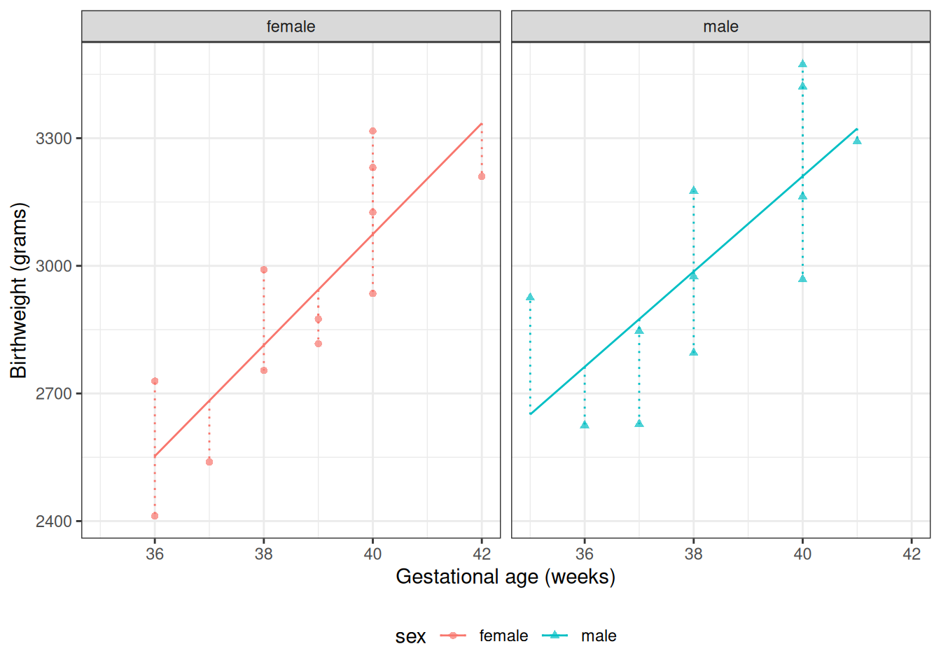
Cook, R. Dennis. 1977. “Detection of Influential Observation in Linear Regression.” Technometrics 19 (1): 15–18. https://doi.org/10.1080/00401706.1977.10489493.
Dobson, Annette J, and Adrian G Barnett. 2018. An Introduction to Generalized Linear Models. 4th ed. CRC press. https://doi.org/10.1201/9781315182780.
Draper, Norman R, and Harry Smith. 2014. Applied Regression Analysis. 3rd ed. John Wiley & Sons. https://www.wiley.com/en-us/Applied+Regression+Analysis%2C+3rd+Edition-p-9781118625682.
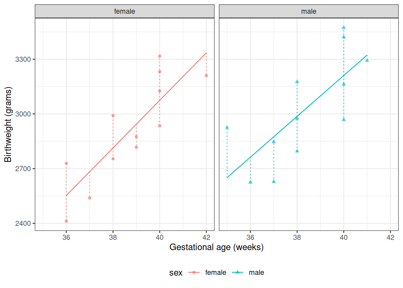
Dunn, Peter K, and Gordon K Smyth. 2018. Generalized Linear Models with Examples in R. Vol. 53. Springer. https://link.springer.com/book/10.1007/978-1-4419-0118-7.
Faraway, Julian J. 2025. Linear Models with R. https://www.routledge.com/Linear-Models-with-R/Faraway/p/book/9781032583983.
Harrell, Frank E. 2015. Regression Modeling Strategies: With Applications to Linear Models, Logistic Regression, and Survival Analysis. 2nd ed. Springer. https://doi.org/10.1007/978-3-319-19425-7.
Heinze, Georg, Christine Wallisch, and Daniela Dunkler. 2018. “Variable Selection – A Review and Recommendations for the Practicing Statistician.” Biometrical Journal 60 (3): 431–49. https://doi.org/10.1002/bimj.201700067.
Hogg, Robert V., Elliot A. Tanis, and Dale L. Zimmerman. 2015. Probability and Statistical Inference. Ninth edition. Pearson.
Hulley, Stephen, Deborah Grady, Trudy Bush, et al. 1998. “Randomized Trial of Estrogen Plus Progestin for Secondary Prevention of Coronary Heart Disease in Postmenopausal Women.” JAMA : The Journal of the American Medical Association (Chicago, IL) 280 (7): 605–13.
James, Gareth, Daniela Witten, Trevor Hastie, Robert Tibshirani, et al. 2013. An Introduction to Statistical Learning. Vol. 112. Springer. https://www.statlearning.com/.
James, Gareth, Daniela Witten, Trevor Hastie, and Robert Tibshirani. 2021. An Introduction to Statistical Learning: With Applications in R. 2nd ed. Springer. https://doi.org/10.1007/978-1-0716-1418-1.
Kleinbaum, David G, and Mitchel Klein. 2010. Logistic Regression: A Self-Learning Text. 3rd ed. Springer. https://link.springer.com/book/10.1007/978-1-4419-1742-3.
Kleinbaum, David G, and Mitchel Klein. 2012. Survival Analysis: A Self-Learning Text. 3rd ed. Springer. https://link.springer.com/book/10.1007/978-1-4419-6646-9.
Kleinbaum, David G, Lawrence L Kupper, Azhar Nizam, K Muller, and ES Rosenberg. 2014. Applied Regression Analysis and Other Multivariable Methods. 5th ed. Cengage Learning. https://www.cengage.com/c/applied-regression-analysis-and-other-multivariable-methods-5e-kleinbaum/9781285051086/.
Kutner, Michael H, Christopher J Nachtsheim, John Neter, and William Li. 2005. Applied Linear Statistical Models. McGraw-Hill.
Polin, Richard A, William W Fox, and Steven H Abman. 2011. Fetal and Neonatal Physiology. 4th ed. Elsevier health sciences.
Schwarz, Gideon. 1978. “Estimating the Dimension of a Model.” The Annals of Statistics 6 (2): 461–64. https://doi.org/10.1214/aos/1176344136.
Seber, George AF, and Alan J Lee. 2012. Linear Regression Analysis. 2nd ed. John Wiley & Sons. https://www.wiley.com/en-us/Linear+Regression+Analysis%2C+2nd+Edition-p-9781118274422.
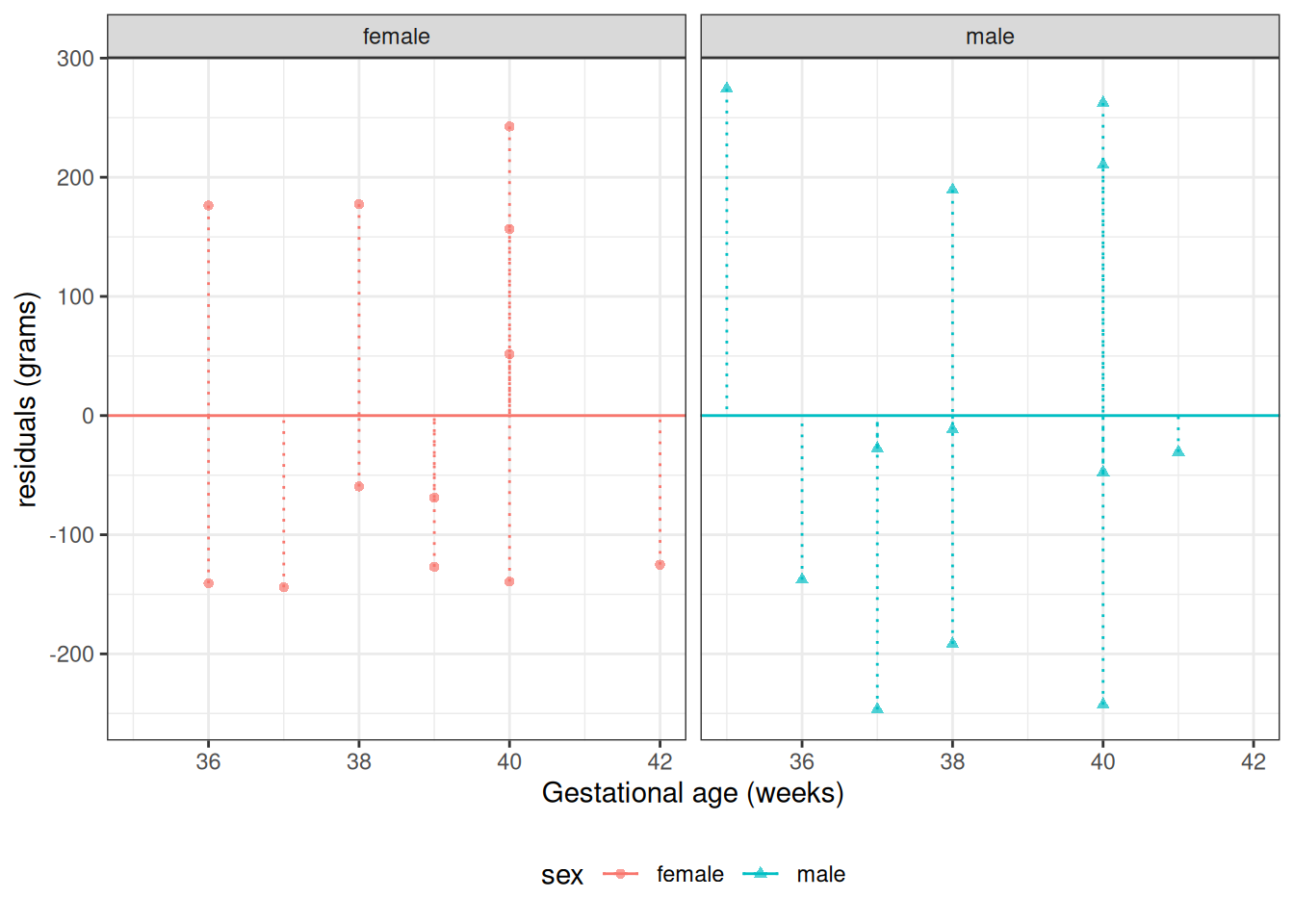
Venables, Bill. 2023. codingMatrices: Alternative Factor Coding Matrices for Linear Model Formulae. Version 0.4.0. https://CRAN.R-project.org/package=codingMatrices.
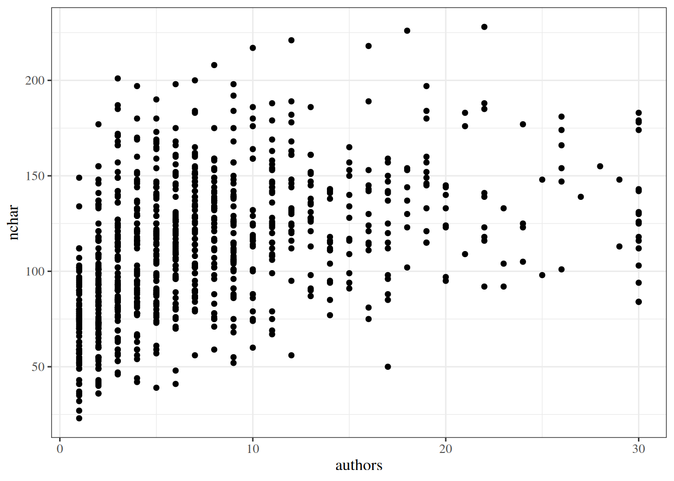
Vittinghoff, Eric, David V Glidden, Stephen C Shiboski, and Charles E McCulloch. 2012. Regression Methods in Biostatistics: Linear, Logistic, Survival, and Repeated Measures Models. 2nd ed. Springer. https://doi.org/10.1007/978-1-4614-1353-0.
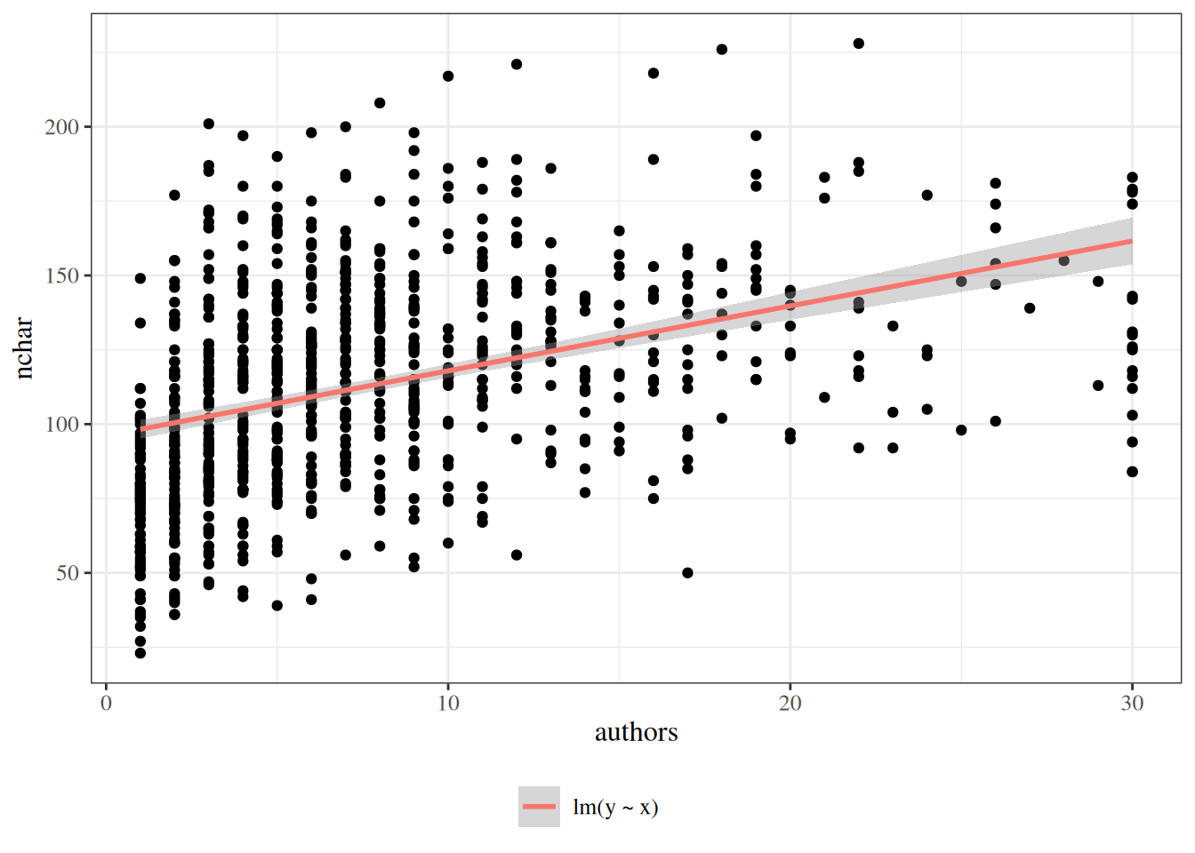
Weisberg, Sanford. 2005. Applied Linear Regression. Vol. 528. John Wiley & Sons.