The following code implements an Expectation-Maximization (EM) algorithm to find the maximum likelihood estimate of the parameters of a two-component Gaussian mixture model.
Problem summary
In statistics, a finite mixture model is a probabilistic model in which each observation comes from one of several latent subpopulations, but the subpopulation labels are not observable.
For example, suppose that you are tying to model the weights of the birds in your local park. The birds belong to two flocks, and those flocks have different feeding grounds, so they have different distributions of weights. However, you don’t know which birds belong to which flock when you catch them for weighing. You would like to estimate the mean weight and standard deviation for each flock, as well as the proportion of caught birds that come from each flock.
Supposed you catch and weigh \(n = 100\) birds, and the recorded weights are \(y_1,...y_n\). Let \(X_i\) represent the flock that bird \(i\) belongs to, with \(X=1\) representing one flock and \(X=2\) representing the other flock.
A mixture model for this data has the structure:
\[p(Y=y) = \sum_{x\in\{1,2\}} p(Y=y|X=x)P(X=x)\]
To complete this model, let’s assume that \(p(Y=y|X=1)\) is a Gaussian (“bell-curve”) distribution with parameters \(\mu_1\) and \(\sigma_1\), and similarly for p(Y=y|X=2)$.
We want to estimate five parameters:
- \(\mu_1 := \text{E}[Y|X=1]\): the average weight of birds in flock 1
- \(\sigma_1 := \text{SD}(Y|X=1)\): the standard deviation of weights among birds in flock 1
- \(\mu_2 := \text{E}[Y|X=2]\): the average weight of birds in flock 2
- \(\sigma_2 := \text{SD}(Y|X=2)\): the standard deviation of weights among birds in flock 2
- \(\pi_1 := P(X=1)\): the proportion of caught birds that belong to flock 12
If we could directly observe the flock membership for each weighed bird, \(x_1,...,x_n\), and count the number tbat came from each flock, \(n_1\) and \(n_2\). Then this would be an easy problem:
- \(\hat{\mu}_1 = \sum_{\{i: x_i = 1\}} Y_i\)
- \(\hat{\sigma}_1 = \sqrt{\frac{1}{n_1} \sum_{\{i: x_i = 1\}}(Y_i - \hat{\mu}_1)^2}\)
- \(\hat{\pi_1} = n_1/n\)
- [similarly for \(\mu_2\) and \(\sigma_2\)]
But what if we can’t observe \(x\)? Can we still estimate \(\mu_1\), \(\mu_2\), \(\sigma_1\), \(\sigma_2\), and \(\pi\)?
If we try to directly maximize the likelihood of the observed data, \(\mathcal{L} = \prod_{i\in 1:n} {p(Y=y_i)}\), by taking the derivative of the log-likelihood \(\ell = \log{\mathcal{L}}\), setting ’ equal to zero, and solving for the parameters, we quickly run into difficulties in taking the derivative of \(\ell\), because \(p(Y=y_i)\) is a sum (try it!).
EM algorithm to the rescue
The EM algorithm is an iterative method for finding the maximum likelihood estimates of parameters in models with latent (unobserved) variables. The Gaussian mixture model in this code assumes that the observed data, \(Y\), is generated from either one of two Gaussian distributions with means \(\mu_1\) and \(mu_2\) and a common standard deviation \(\sigma\). The probability of the data coming from the first Gaussian distribution is \(\pi\), while the probability of the data coming from the second Gaussian distribution is \(1 - \pi\).
The gen_data() function generates data according to this
Gaussian mixture model, while the fit_model() function
performs the EM algorithm. The E_step function calculates the expected
value of the log-likelihood given the current estimates of the
parameters and the observed data, while the M_step updates the estimates
of the parameters based on the expected log-likelihood. The algorithm
continues to iterate until the difference in the log-likelihood between
consecutive iterations is less than a specified tolerance (tolerance).
The results of the algorithm are saved in a progress tibble that shows
the values of the estimated parameter pi-hat and the log-likelihood for
each iteration.
Generate data
gen_data = function(
    n = 500000,
    mu = c(0,2),
    sigma = 1,
    pi = 0.8)
{

  tibble(
    Obs.ID = 1:n,
    Z = (runif(n) > pi) + 1,
    Y = rnorm(n = n, mean = mu[Z], sd = sigma)
  ) |>
    select(-Z) |>
    mutate(
      `p(Y=y|Z=1)` = dnorm(Y, mu[1], sd = sigma),
      `p(Y=y|Z=2)` = dnorm(Y, mu[2], sd = sigma),
    )

}| Obs.ID | Y | p(Y=y|Z=1) | p(Y=y|Z=2) |
|---|---|---|---|
| 1 | 0.2415 | 0.3875 | 0.08499 |
| 2 | -0.4071 | 0.3672 | 0.02202 |
| 3 | 0.01312 | 0.3989 | 0.05542 |
| 4 | 2.756 | 0.008952 | 0.2999 |
| 5 | -0.4597 | 0.3589 | 0.01937 |
| 6 | 1.505 | 0.1286 | 0.3529 |
Fit model
fit_model = function(
    data,
    `p(Z=1)` = 0.5, # initial guess for `pi-hat`
    tolerance = 0.00001,
    max_iterations = 1000,
    verbose = FALSE
)
{

  # pre-allocate a table of results by iteration:
  progress = tibble(
      Iteration = 0:max_iterations,
      `p(Z=1)` = NA_real_,
      loglik =  NA_real_,
      diff_loglik = NA_real_
    )

  # initial E step, to perform needed calculations for initial likelihood:
  data = data |> E_step(`p(Z=1)` = `p(Z=1)`)
  ll = loglik(data)
  progress[1, ] = list(0, `p(Z=1)`, ll, NA)

  for(i in 1:max_iterations)
  {
    # M step: re-estimate parameters
    `p(Z=1)` = data |> M_step()

    # E step: re-compute distribution of missing variables, using parameters
    data = data |> E_step(`p(Z=1)` = `p(Z=1)`)

    # Assess convergence

    ## save the previous log-likelihood so we can test for convergence
    ll_old = ll

    ## here's the new log-likelihood
    ll = loglik(data)

    ll_diff = ll - ll_old

    progress[i+1, ] = list(i, `p(Z=1)`, ll, ll_diff)

    if(verbose) print(progress[i+1, ])

    if(ll_diff < tolerance) break;
  }

  return(progress[1:(i+1), ])
}
E step
E_step = function(data, `p(Z=1)`)
{
  data |>
    mutate(
      `p(Y=y, Z=1)` = `p(Y=y|Z=1)` * `p(Z=1)`,
      `p(Y=y, Z=2)` = `p(Y=y|Z=2)` * (1 - `p(Z=1)`),
      `p(Y=y)`      = `p(Y=y, Z=1)` + `p(Y=y, Z=2)`,
      `p(Z=1|Y=y)`  = `p(Y=y, Z=1)` / `p(Y=y)`,
    )
}Results
Finally, the system.time() function is used to measure
the time it takes to run the fit_model() function:
{results = fit_model(data, tolerance = 0.00001)} |>
  system.time()
#>    user  system elapsed
#>   0.437   0.031   0.468
print(results, n = Inf)
#> # A tibble: 19 × 4
#> Iteration `p(Z=1)` loglik diff_loglik
#> <int> <dbl> <dbl> <dbl>
#> 1 0 0.5 -877590. NA
#> 2 1 0.665 -837000. 4.06e+4
#> 3 2 0.738 -828034. 8.97e+3
#> 4 3 0.770 -825959. 2.07e+3
#> 5 4 0.785 -825455. 5.05e+2
#> 6 5 0.793 -825328. 1.27e+2
#> 7 6 0.797 -825295. 3.24e+1
#> 8 7 0.799 -825287. 8.36e+0
#> 9 8 0.800 -825285. 2.17e+0
#> 10 9 0.800 -825284. 5.63e-1
#> 11 10 0.800 -825284. 1.46e-1
#> 12 11 0.800 -825284. 3.81e-2
#> 13 12 0.800 -825284. 9.92e-3
#> 14 13 0.801 -825284. 2.58e-3
#> 15 14 0.801 -825284. 6.73e-4
#> 16 15 0.801 -825284. 1.75e-4
#> 17 16 0.801 -825284. 4.56e-5
#> 18 17 0.801 -825284. 1.19e-5
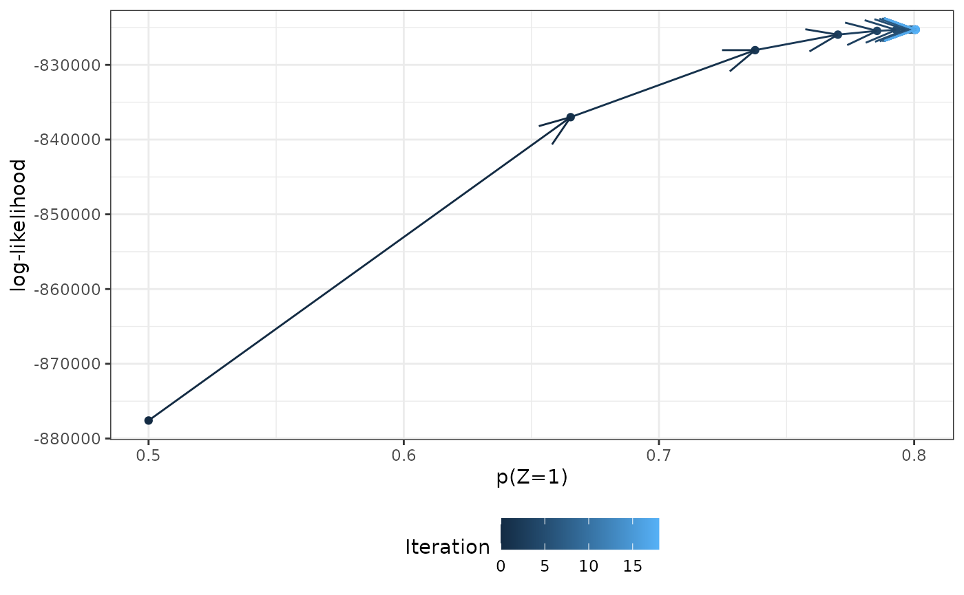
#> 19 18 0.801 -825284. 3.09e-6Here’s what happened:
library(ggplot2)
results |>
  ggplot(aes(
    x = `p(Z=1)`,
    y = loglik,
    col = Iteration
  )) +
  geom_point() +
  geom_path(
    arrow = arrow(
    angle = 20,
      type = "open"
  )) +
  theme_bw() +
  ylab("log-likelihood") +
  theme(
    legend.position = "bottom"
  )