Proportional Hazards Models

Configuring R

Functions from these packages will be used throughout this document:

library(conflicted) # check for conflicting function definitions
# library(printr) # inserts help-file output into markdown output
library(rmarkdown) # Convert R Markdown documents into a variety of formats.
library(pander) # format tables for markdown
library(ggplot2) # graphics
library(ggfortify) # help with graphics
library(dplyr) # manipulate data
library(tibble) # `tibble`s extend `data.frame`s
library(magrittr) # `%>%` and other additional piping tools
library(haven) # import Stata files
library(knitr) # format R output for markdown
library(tidyr) # Tools to help to create tidy data
library(plotly) # interactive graphics
library(dobson) # datasets from Dobson and Barnett 2018
library(parameters) # format model output tables for markdown
library(haven) # import Stata files
library(latex2exp) # use LaTeX in R code (for figures and tables)
library(fs) # filesystem path manipulations
library(survival) # survival analysis
library(survminer) # survival analysis graphics
library(KMsurv) # datasets from Klein and Moeschberger
library(parameters) # format model output tables for
library(webshot2) # convert interactive content to static for pdf
library(forcats) # functions for categorical variables ("factors")
library(stringr) # functions for dealing with strings
library(lubridate) # functions for dealing with dates and times

Here are some R settings I use in this document:

rm(list = ls()) # delete any data that's already loaded into R

conflicts_prefer(dplyr::filter)
ggplot2::theme_set(
  ggplot2::theme_bw() + 
        # ggplot2::labs(col = "") +
    ggplot2::theme(
      legend.position = "bottom",
      text = ggplot2::element_text(size = 12, family = "serif")))

knitr::opts_chunk$set(message = FALSE)
options('digits' = 6)

panderOptions("big.mark", ",")
pander::panderOptions("table.emphasize.rownames", FALSE)
pander::panderOptions("table.split.table", Inf)
conflicts_prefer(dplyr::filter) # use the `filter()` function from dplyr() by default
legend_text_size = 9
run_graphs = TRUE

1 Introduction

Exercise 1 Recall the key characteristics of the exponential distribution:

• density function \(\text{f}(t)\)
• survival function \(\text{S}(t)\)
• hazard function \({\lambda}(t)\)

Solution 1. \[ \begin{aligned} \text{p}(t) &= \lambda e^{-\lambda t}\\ \text{S}(t) &= e^{-\lambda t}\\ {\lambda}(t) &= \lambda \end{aligned} \]

Note that the exponential distribution has constant hazard.

2 Understanding proportional hazards models

Let’s make two generalizations. First, we let the hazard depend on some covariates \(x_1,x_2, \dots, x_p\); we will indicate this dependence by extending our notation for hazard:

Definition 1 (conditional hazard) The conditional hazard of outcome \(T\) at value \(t\), given covariate vector \(\tilde{x}\), is the conditional density of the event \(T=t\), given \(T \ge t\) and \(\tilde{X}= \tilde{x}\):

\[{\lambda}(t|\tilde{x}) \stackrel{\text{def}}{=}\text{p}(T=t|T\ge t, \tilde{X}= \tilde{x}) \tag{1}\]

Definition 2 (baseline hazard)  

The baseline hazard, base hazard, or reference hazard, denoted \({\lambda}_0(t)\) or \(\lambda_0(t)\), is the hazard function for the subpopulation of individuals whose covariates are all equal to their reference levels:

\[{\lambda}_0(t) \stackrel{\text{def}}{=}{\lambda}(t | \tilde{X}= \tilde{0}) \tag{2}\]

The baseline hazard is somewhat analogous to the intercept term in linear regression, but it is not a mean.

Similarly:

Definition 3 (baseline cumulative hazard)  

The baseline cumulative hazard, base cumulative hazard, or reference cumulative hazard, denoted \(H_0(t)\) or \(\Lambda_0(t)\), is the cumulative hazard function for the subpopulation of individuals whose covariates are all equal to their reference levels:

\[{\Lambda}_0(t) \stackrel{\text{def}}{=}{\Lambda}(t | \tilde{X}= \tilde{0}) \tag{3}\]

Also:

Definition 4 (Baseline survival function) The baseline survival function is the survival function for an individual whose covariates are all equal to their default values.

\[\text{S}_0(t) \stackrel{\text{def}}{=}\text{S}(t | \tilde{X}= \tilde{0})\]

Now, let’s define how the hazard function depends on covariates. We typically use a log link to model the relationship between the hazard function, \({\lambda}(t|\tilde{x})\), and the linear component, \(\eta(t|\tilde{x})\), as we did for Poisson models in models for count outcomes; that is:

Definition 5 (log-hazard)  

The log-hazard function, denoted \(\eta(t)\), is the natural logarithm of the hazard function:

\[\eta(t) \stackrel{\text{def}}{=}\text{log}{\left\{{\lambda}(t)\right\}}\]

Definition 6 (conditional log-hazard)  

The conditional log-hazard function, denoted \(\eta(t|\tilde{x})\), is the natural logarithm of the conditional hazard function:

\[\eta(t | \tilde{x}) \stackrel{\text{def}}{=}\text{log}{\left\{{\lambda}(t | \tilde{x})\right\}}\]

In contrast with Poisson regression, here \(\eta(t|\tilde{x})\) depends on both \(t\) and \(\tilde{x}\).

Definition 7 (baseline log-hazard)  

The baseline log-hazard, denoted \(\eta_0(t)\), log-hazard function for the subpopulation of individuals whose covariates are all equal to their reference levels:

\[\eta_0(t) \stackrel{\text{def}}{=}\eta(t | \tilde{X}= \tilde{0})\]

Theorem 1 \[ \begin{aligned} {\lambda}(t|\tilde{x}) &= \text{exp}{\left\{\eta(t|\tilde{x})\right\}} \end{aligned} \]

Definition 8 (difference in log-hazards) The difference in log-hazards between covariate patterns \(\tilde{x}\) and \({\tilde{x}^*}\) at time \(t\) is:

\[\Delta \eta(t|\tilde{x}: {\tilde{x}^*}) \stackrel{\text{def}}{=}\eta(t|\tilde{x}) - \eta(t|{\tilde{x}^*})\]

Theorem 2 (Difference of log-hazards vs hazard ratio) If \(\Delta \eta(t|\tilde{x}: {\tilde{x}^*})\) is the difference in log-hazard between covariate patterns \(\tilde{x}\) and \({\tilde{x}^*}\) at time \(t\), and \(\theta(t| \tilde{x}: {\tilde{x}^*})\) is corresponding hazard ratio, then:

\[\Delta \eta(t|\tilde{x}: {\tilde{x}^*})= \text{log}{\left\{\theta(t| \tilde{x}: {\tilde{x}^*})\right\}}\]

Proof. Using the hazard ratio definition:

\[ \begin{aligned} \Delta \eta(t|\tilde{x}: {\tilde{x}^*}) &\stackrel{\text{def}}{=}\eta(t|\tilde{x}) - \eta(t|{\tilde{x}^*}) \\ &= \text{log}{\left\{{\lambda}(t|\tilde{x})\right\}} - \text{log}{\left\{{\lambda}(t|{\tilde{x}^*})\right\}} \\ &= \text{log}{\left\{\frac{{\lambda}(t|\tilde{x})}{{\lambda}(t|{\tilde{x}^*})}\right\}} \\ &= \text{log}{\left\{\theta(t| \tilde{x}: {\tilde{x}^*})\right\}} \end{aligned} \]

Corollary 1 (Hazard ratio vs difference of log-odds) \[\theta(t| \tilde{x}: {\tilde{x}^*}) = \text{exp}{\left\{\Delta \eta(t|\tilde{x}: {\tilde{x}^*})\right\}}\]

Definition 9 (difference in log-hazard from baseline)  

The difference in log-hazard for covariate pattern \(\tilde{x}\) compared to the baseline covariate pattern \(\tilde{0}\) is:

\[ \begin{aligned} \Delta \eta(t|\tilde{x}) &\stackrel{\text{def}}{=}\Delta \eta(t | \tilde{x}: \tilde{0}) \end{aligned} \]

Theorem 3 (Decomposition of log-hazard) \[ \begin{aligned} \eta(t|\tilde{x}) = \eta_0(t) + \Delta \eta(t|\tilde{x}) \end{aligned} \]

Definition 10 (Hazard ratio versus baseline) \[\theta(t|\tilde{x}) \stackrel{\text{def}}{=}\theta(t| \tilde{x}: \tilde{0}) \tag{4}\]

Corollary 2 \[\theta(t|\tilde{x})= \text{exp}{\left\{\Delta \eta(t|\tilde{x})\right\}}\]

Proof. \[ \begin{aligned} \theta(t|\tilde{x}) &\stackrel{\text{def}}{=}\theta(t| \tilde{x}: \tilde{0}) \\ &= \text{exp}{\left\{\Delta \eta(t|\tilde{x})\right\}} \end{aligned} \]

Corollary 3 \[\Delta \eta(t|\tilde{x}) = \text{log}{\left\{\theta(t| \tilde{x})\right\}}\]

As the second generalization, we let the base hazard, cumulative hazard, and survival functions depend on \(t\), but not on any covariates (for now). We can do this using either parametric or semi-parametric approaches.

Definition 11 (Proportional hazards model) A proportional hazards model for a time-to-event outcome \(T\) is a model where the difference in log-hazard from the baseline log-hazard is equal to a linear combination of the predictors:

\[\Delta \eta(t|\tilde{x}) = \tilde{x}\cdot \tilde{\beta} \tag{5}\]

Equivalently:

Lemma 1 In a proportional hazards model (that is, if Equation 5 holds):

\[ \begin{aligned} \eta(t|\tilde{x}) &= \eta_0(t) + \tilde{x}\cdot \tilde{\beta} \\ &= \eta_0(t) + \beta_1 x_1+ \dots + \beta_p x_p \end{aligned} \tag{6}\]

In a proportional hazards model, the baseline log-hazard is analogous to the intercept term in a generalized linear model, except that the baseline log-hazard depends on time, \(t\).

Lemma 2 If \(\eta(t|\tilde{x}) = \eta_0(t) + \tilde{x}\cdot \tilde{\beta}\), then:

\[ \begin{aligned} \Delta \eta(t|\tilde{x}: {\tilde{x}^*}) &= (\tilde{x}- {\tilde{x}^*}) \cdot \beta \end{aligned} \]

Theorem 4 If \(\eta(t|\tilde{x}) = \eta_0(t) + \tilde{x}\cdot \tilde{\beta}\), then:

\[ \begin{aligned} \theta(t|\tilde{x}: {\tilde{x}^*}) &= \text{exp}{\left\{\Delta \eta(t|\tilde{x}: {\tilde{x}^*})\right\}} \\ &= \text{exp}{\left\{(\tilde{x}- {\tilde{x}^*}) \cdot \beta\right\}} \end{aligned} \]

So for proportional hazards models, we can write the hazard ratio using a shorthand notation:

\[\theta(t| \tilde{x}: {\tilde{x}^*}) = \theta(\tilde{x}: {\tilde{x}^*})\]

Lemma 3 \[\Delta \eta(t|\tilde{x})= \tilde{x}\cdot \tilde{\beta} \tag{7}\]

Theorem 5 If \(\eta(t|\tilde{x}) = \eta_0(t) + \tilde{x}\cdot \tilde{\beta}\), then:

\[\theta(t|\tilde{x}) = \text{exp}{\left\{\tilde{x}\cdot \tilde{\beta}\right\}}\]

Proof. \[ \begin{aligned} \theta(t|\tilde{x}) &\stackrel{\text{def}}{=}\theta(t| \tilde{x}: \tilde{0}) \\ &= \text{exp}{\left\{\Delta \eta(t|\tilde{x})\right\}} \\ &= \text{exp}{\left\{\tilde{x}\cdot \tilde{\beta}\right\}} \end{aligned} \]

Theorem 6 \[{\lambda}(t|x) = {\lambda}_0(t)\theta(x)\]

Also:

Theorem 7 \[ \begin{aligned} \theta(x) &= \text{exp}{\left\{\Delta \eta(x)\right\}} \\ \log{{\lambda}(t|x)} &= \log{{\lambda}_0(t)} + \Delta \eta(x) \\ &= \eta_0(t) + \Delta \eta(x) \\ \Delta \eta(x) &= \tilde{x}\cdot \tilde{\beta}\\ &\stackrel{\text{def}}{=}\beta_1x_1+\cdots+\beta_px_p \end{aligned} \]

This model is semi-parametric, because the linear predictor depends on estimated parameters but the base hazard function is unspecified. There is no constant term in \(\eta(x)\), because it is absorbed in the base hazard.

Alternatively, we could define \(\beta_0(t) = \log{{\lambda}_0(t)}\), and then:

\[\eta(x,t) = \beta_0(t) + \beta_1x_1+\cdots+\beta_px_p\]

For two different individuals with covariate patterns \(\tilde{x}_1\) and \(\tilde{x}_2\), the ratio of the hazard functions (a.k.a. hazard ratio, a.k.a. relative hazard) is:

\[ \begin{aligned} \frac{{\lambda}(t|\tilde{x}_1)}{{\lambda}(t|\tilde{x}_2)} &=\frac{{\lambda}_0(t)\theta(\tilde{x}_1)}{{\lambda}_0(t)\theta(\tilde{x}_2)}\\ &=\frac{\theta(\tilde{x}_1)}{\theta(\tilde{x}_2)}\\ \end{aligned} \]

Under the proportional hazards model, this ratio (a.k.a. proportion) does not depend on \(t\). This property is a structural limitation of the model; it is called the proportional hazards assumption.

Definition 12 (proportional hazards) A conditional probability distribution \(p(T|X)\) has proportional hazards if the hazard ratio \({\lambda}(t|\tilde{x}_1)/{\lambda}(t|\tilde{x}_2)\) does not depend on \(t\). Mathematically, it can be written as:

\[ \frac{{\lambda}(t|\tilde{x}_1)}{{\lambda}(t|\tilde{x}_2)} = \theta(\tilde{x}_1,\tilde{x}_2) \]

As we saw above, Cox’s proportional hazards model has this property, with \(\theta(\tilde{x}_1,\tilde{x}_2) = \frac{\theta(\tilde{x}_1)}{\theta(\tilde{x}_2)}\).

Theorem 8  

We are using two similar notations, \(\theta(\tilde{x},{\tilde{x}^*})\) and \(\theta(\tilde{x})\). We can link these notations: \[\theta(\tilde{x}) \stackrel{\text{def}}{=}\theta(\tilde{x}, \tilde{0})\]

Then:

\[\theta(\tilde{x}, {\tilde{x}^*}) = \frac{\theta(\tilde{x})}{\theta({\tilde{x}^*})}\] \[\theta(\tilde{0}) = \theta(\tilde{0}, \tilde{0}) = 1\]

The proportional hazards model also has additional notable properties:

\[ \begin{aligned} \frac{{\lambda}(t|\tilde{x}_1)}{{\lambda}(t|\tilde{x}_2)} &=\frac{\theta(\tilde{x}_1)}{\theta(\tilde{x}_2)}\\ &=\frac{\text{exp}{\left\{\eta(\tilde{x}_1)\right\}}}{\text{exp}{\left\{\eta(\tilde{x}_2)\right\}}}\\ &=\text{exp}{\left\{\eta(\tilde{x}_1)-\eta(\tilde{x}_2)\right\}}\\ &=\text{exp}{\left\{\tilde{x}_1'\beta-\tilde{x}_2'\beta\right\}}\\ &=\text{exp}{\left\{(\tilde{x}_1 - \tilde{x}_2)'\beta\right\}}\\ \end{aligned} \]

Hence on the log scale, we have:

Theorem 9 \[ \begin{aligned} \log{\frac{{\lambda}(t|\tilde{x})}{{\lambda}(t|{\tilde{x}^*})}} &= \Delta \eta(t|\tilde{x}: {\tilde{x}^*}) \\ &\stackrel{\text{def}}{=}\eta(t|\tilde{x}) - \eta(t|{\tilde{x}^*}) \\ &=\eta(\tilde{x}_1)-\eta(\tilde{x}_2)\\ &= \tilde{x}_1'\beta-\tilde{x}_2'\beta\\ &= (\tilde{x}_1 - \tilde{x}_2)'\beta \end{aligned} \]

If only one covariate \(x_j\) is changing, then:

\[ \begin{aligned} \log{\frac{{\lambda}(t|\tilde{x}_1)}{{\lambda}(t|\tilde{x}_2)}} &= (x_{1j} - x_{2j}) \cdot \beta_j\\ &\propto (x_{1j} - x_{2j}) \end{aligned} \]

That is, under Cox’s model \({\lambda}(t|\tilde{x}) = {\lambda}_0(t)\text{exp}{\left\{\tilde{x}'\beta\right\}}\), the log of the hazard ratio is proportional to the difference in \(x_j\), with the proportionality coefficient equal to \(\beta_j\).

Further,

\[ \begin{aligned} \log{{\lambda}(t|\tilde{x})} &=\log{{\lambda}_0(t)} + x'\beta \end{aligned} \]

That is, the covariate effects are additive on the log-hazard scale; hazard functions for different covariate patterns should be vertical shifts of each other.

See also:

https://en.wikipedia.org/wiki/Proportional_hazards_model#Why_it_is_called_%22proportional%22

Additional properties of the proportional hazards model

If \({\lambda}(t|x)= {\lambda}_0(t)\theta(x)\), then:

Theorem 10 (Cumulative hazards are also proportional to \({\Lambda}_0(t)\)) \[ \begin{aligned} {\Lambda}(t|x) &\stackrel{\text{def}}{=}\int_{u=0}^t {\lambda}(u)du\\ &= \int_{u=0}^t {\lambda}_0(u)\theta(x)du\\ &= \theta(x)\int_{u=0}^t {\lambda}_0(u)du\\ &= \theta(x){\Lambda}_0(t) \end{aligned} \]

where \({\Lambda}_0(t) \stackrel{\text{def}}{=}{\Lambda}(t|0) = \int_{u=0}^t {\lambda}_0(u)du\).

Theorem 11 (The logarithms of cumulative hazard should be parallel) \[ \text{log}{\left\{{\Lambda}(t|\tilde{x})\right\}} =\text{log}{\left\{{\Lambda}_0(t)\right\}} + \tilde{x}\cdot \tilde{\beta} \]

Corollary 4 (linear model for log-negative-log survival) \[ \text{log}{\left\{-\text{log}{\left\{\text{S}(t|\tilde{x})\right\}}\right\}} = \text{log}{\left\{-\text{log}{\left\{\text{S}_0(t)\right\}}\right\}} + \tilde{x}\cdot \tilde{\beta} \]

Theorem 12 (Survival functions are exponential multiples of \(\text{S}_0(t)\)) \[\text{S}(t|x) = {\left[\text{S}_0(t)\right]}^{\theta(x)}\]

Proof. \[ \begin{aligned} \text{S}(t|x) &= \text{exp}{\left\{-{\Lambda}(t|x)\right\}}\\ &= \text{exp}{\left\{-\theta(x)\cdot {\Lambda}_0(t)\right\}}\\ &= {\left(\text{exp}{\left\{- {\Lambda}_0(t)\right\}}\right)}^{\theta(x)}\\ &= {\left[\text{S}_0(t)\right]}^{\theta(x)}\\ \end{aligned} \]

Summary of proportional hazards model structure and assumptions

Joint likelihood of data set: \(\mathscr{L}\stackrel{\text{def}}{=}\text{p}(\tilde{Y}= \tilde{y}, \tilde{D}= \tilde{d}| \mathbf{X}= \mathbf{x})\)

Marginal likelihood contribution of obs. i : \(\mathscr{L}_i \stackrel{\text{def}}{=}\text{p}(Y_i= y_i, D_i = d_i | \tilde{X}_i = \tilde{x}_i)\)

Independent Observations Assumption: \(\mathscr{L}= \prod_{i=1}^n \mathscr{L}_i\)

Non-Informative Censoring Assumption: \(T_i\perp\!\!\!\perp C_i | \tilde{X}_i\)

\[ \mathscr{L}_i \propto [\text{f}_T(y_i|\tilde{x}_i)]^{d_i} [\text{S}_T(y_i | \tilde{x}_i)]^{1-d_i} = \text{S}_T(y_i|\tilde{x}_i) \cdot [{\lambda}_T(y_i|\tilde{x}_i)]^{d_i} \]

Survival function: \(\text{S}(t | \tilde{x}) \stackrel{\text{def}}{=}\text{P}(T > t|\tilde{X}= \tilde{x}) = \int_{u=t}^{\infty} \text{f}(u|\tilde{x})du = \text{exp}{\left\{-{\Lambda}(t|\tilde{x})\right\}}\)

Probability density function: \(\text{f}(t| \tilde{x}) \stackrel{\text{def}}{=}\text{p}(T=t|\tilde{X}= \tilde{x}) = -\text{S}'(t|\tilde{x}) = {\lambda}(t| \tilde{x}) \text{S}(t | \tilde{x})\)

Cumulative hazard function: \({\Lambda}(t | \tilde{x}) \stackrel{\text{def}}{=}\int_{u=0}^t {\lambda}(u|\tilde{x})du = -\text{log}{\left\{\text{S}(t|\tilde{x})\right\}}\)

Hazard function: \({\lambda}(t |\tilde{x}) \stackrel{\text{def}}{=}\text{p}(T=t|T\ge t,\tilde{X}= \tilde{x}) = {\Lambda}'(t|\tilde{x}) = \frac{\text{f}(t|\tilde{x})}{\text{S}(t|\tilde{x})}\)

Hazard ratio: \(\theta(t| \tilde{x}: {\tilde{x}^*}) \stackrel{\text{def}}{=}\frac{{\lambda}(t|\tilde{x})}{{\lambda}(t|{\tilde{x}^*})}\)

Log-Hazard function: \(\eta(t|\tilde{x}) \stackrel{\text{def}}{=}\text{log}{\left\{\lambda(t|\tilde{x})\right\}} = \eta_0(t) + \Delta \eta(t|\tilde{x})\)

Proportional Hazards Assumption:

\[ \begin{aligned} {\lambda}(t |\tilde{x}) &= {\lambda}_0(t) \cdot \theta(\tilde{x}) \\ {\Lambda}(t |\tilde{x}) &= {\Lambda}_0(t) \cdot \theta(\tilde{x}) \\ \eta(t|\tilde{x}) &= \eta_0(t) + \Delta \eta(\tilde{x}) \end{aligned} \]

Logarithmic Link Function Assumption:

• Link function: \[\text{log}{\left\{{\lambda}(t|\tilde{x})\right\}} = \eta(t|\tilde{x})\] \[\text{log}{\left\{\theta(\tilde{x})\right\}} = \Delta \eta(\tilde{x})\]

• Inverse link function: \[{\lambda}(t|\tilde{x}) = \text{exp}{\left\{\eta(t|\tilde{x})\right\}}\] \[\theta(\tilde{x}) = \text{exp}{\left\{\Delta \eta(\tilde{x})\right\}}\]

Linear Predictor Component:

\[\eta(t|\tilde{x}) = \eta_0(t) + \Delta \eta(t|\tilde{x})\] \[\Delta \eta(t|\tilde{x}) = \tilde{x}\cdot \tilde{\beta}\]

Linear Predictor Component Functional Form Assumption:

\[\Delta \eta(t|\tilde{x}) = \tilde{x}\cdot \tilde{\beta}\stackrel{\text{def}}{=}\beta_1 x_1 + \cdots + \beta_p x_p\]

3 Testing the proportional hazards assumption

The Nelson-Aalen estimate of the cumulative hazard is usually used for estimates of the hazard and often the cumulative hazard.

If the hazards of the three groups are proportional, that means that the ratio of the hazards is constant over \(t\). We can test this using the ratios of the estimated cumulative hazards, which also would be proportional, as shown above.

library(KMsurv)
library(survival)
library(dplyr)
data(bmt)

bmt =
  bmt |>
  as_tibble() |>
  mutate(
    group =
      group |>
      factor(
        labels = c("ALL","Low Risk AML","High Risk AML")))

nafit = survfit(
  formula = Surv(t2,d3) ~ group,
  type = "fleming-harrington",
  data = bmt)

bmt_curves = tibble(timevec = 1:1000)
sf1 <- with(nafit[1], stepfun(time,c(1,surv)))
sf2 <- with(nafit[2], stepfun(time,c(1,surv)))
sf3 <- with(nafit[3], stepfun(time,c(1,surv)))

bmt_curves =
  bmt_curves |>
  mutate(
    cumhaz1 = -log(sf1(timevec)),
    cumhaz2 = -log(sf2(timevec)),
    cumhaz3 = -log(sf3(timevec)))

library(ggplot2)
bmt_rel_hazard_plot =
  bmt_curves |>
  ggplot(
    aes(
      x = timevec,
      y = cumhaz1/cumhaz2)
  ) +
  geom_line(aes(col = "ALL/Low Risk AML")) +
  ylab("Hazard Ratio") +
  xlab("Time") +
  ylim(0,6) +
  geom_line(aes(y = cumhaz3/cumhaz1, col = "High Risk AML/ALL")) +
  geom_line(aes(y = cumhaz3/cumhaz2, col = "High Risk AML/Low Risk AML")) +
  theme_bw() +
  labs(colour = "Comparison") +
  theme(legend.position="bottom")

print(bmt_rel_hazard_plot)

Figure 1: Hazard Ratios by Disease Group for bmt data

We can zoom in on the first 300 days to take a closer look:

bmt_rel_hazard_plot + xlim(c(0,300))

Figure 2: Hazard Ratios by Disease Group (0-300 Days)

The cumulative hazard curves should also be proportional

library(ggfortify)
plot_cuhaz_bmt =
  bmt |>
  survfit(formula = Surv(t2, d3) ~ group) |>
  autoplot(fun = "cumhaz",
           mark.time = TRUE) +
  ylab("Cumulative hazard")

plot_cuhaz_bmt |> print()

Figure 3: Disease-Free Cumulative Hazard by Disease Group

plot_cuhaz_bmt +
  scale_y_log10() +
  scale_x_log10()

Figure 4: Disease-Free Cumulative Hazard by Disease Group (log-scale)

Smoothed hazard functions

The Nelson-Aalen estimate of the cumulative hazard is usually used for estimates of the hazard. Since the hazard is the derivative of the cumulative hazard, we need a smooth estimate of the cumulative hazard, which is provided by smoothing the step-function cumulative hazard.

The R package muhaz handles this for us. What we are looking for is whether the hazard function is more or less the same shape, increasing, decreasing, constant, etc. Are the hazards “proportional”?

library(muhaz)

muhaz(bmt$t2,bmt$d3,bmt$group=="High Risk AML") |> plot(lwd=2,col=3)
muhaz(bmt$t2,bmt$d3,bmt$group=="ALL") |> lines(lwd=2,col=1)
muhaz(bmt$t2,bmt$d3,bmt$group=="Low Risk AML") |> lines(lwd=2,col=2)
legend("topright",c("ALL","Low Risk AML","High Risk AML"),col=1:3,lwd=2)

Figure 5: Smoothed Hazard Rate Estimates by Disease Group

Group 3 was plotted first because it has the highest hazard.

Except for an initial blip in the high risk AML group, the hazards look roughly proportional. They are all strongly decreasing.

4 Fitting proportional hazards models to data

How do we fit a proportional hazards regression model? We need to estimate the coefficients of the covariates, and we need to estimate the base hazard \({\lambda}_0(t)\). For the covariates, supposing for simplicity that there are no tied event times, let the event times for the whole data set be \(t_1, t_2,\ldots,t_D\). Let the risk set at time \(t_i\) be \(R(t_i)\) and

\[ \begin{aligned} \eta(\tilde{x}) &= \beta_1x_{1}+\cdots+\beta_p x_{p}\\ \theta(\tilde{x}) &= e^{\eta(\tilde{x})}\\ {\lambda}(t|X=x)&= {\lambda}_0(t)e^{\eta(\tilde{x})}=\theta(\tilde{x}) {\lambda}_0(t) \end{aligned} \]

Conditional on a single failure at time \(t\), the probability that the event is due to subject \(f\in R(t)\) is approximately

\[ \begin{aligned} \Pr(f \text{ fails}|\text{1 failure at } t) &= \frac{{\lambda}_0(t)e^{\eta(\tilde{x}_f)}}{\sum_{k \in R(t)}{\lambda}_0(t)e^{\eta(\tilde{x}_f)}}\\ &=\frac{\theta(\tilde{x}_f)}{\sum_{k \in R(t)} \theta(\tilde{x}_k)} \end{aligned} \]

The logic behind this has several steps. We first fix (ex post) the failure times and note that in this discrete context, the probability \(p_j\) that a subject \(j\) in the risk set fails at time \(t\) is just the hazard of that subject at that time.

If all of the \(p_j\) are small, the chance that exactly one subject fails is

\[ \sum_{k\in R(t)}p_k\left[\prod_{m\in R(t), m\ne k} (1-p_m)\right]\approx\sum_{k\in R(t)}p_k \]

If subject \(i\) is the one who experiences the event of interest at time \(t_i\), then the partial likelihood is

\[ \begin{aligned} \mathscr{L}^*_i &= \frac{\theta(\tilde{x}_i)}{\sum_{k \in R(t_i)} \theta(\tilde{x}_k)} \\ \mathscr{L}^* &= \prod_{{\left\{i:\ d_i = 1\right\}}} \mathscr{L}^*_i \end{aligned} \]

and we can numerically maximize this with respect to the coefficients \(\tilde{\beta}\) that specify \(\eta(\tilde{x}) = \tilde{x}'\tilde{\beta}\). When there are tied event times adjustments need to be made, but the likelihood is still similar. Note that we don’t need to know the base hazard to solve for the coefficients.

Once we have coefficient estimates \(\hat{\tilde{\beta}} =(\hat \beta_1,\ldots,\hat\beta_p)\), this also defines \(\hat\eta(x)\) and \(\hat\theta(x)\), and then the estimated base cumulative hazard function is

\[\hat {\Lambda}_0(t) = \sum_{t_i < t} \frac{d_i}{\sum_{k\in R(t_i)} \theta(x_k)}\]

which reduces to the Nelson-Aalen estimate when there are no covariates. There are numerous other estimates that have been proposed as well.

5 Example: Proportional hazards model for the bmt data

Fit the model

library(survival)
bmt.cox <- coxph(Surv(t2, d3) ~ group, data = bmt)
summary(bmt.cox)
#> Call:
#> coxph(formula = Surv(t2, d3) ~ group, data = bmt)
#> 
#>   n= 137, number of events= 83 
#> 
#>                      coef exp(coef) se(coef)     z Pr(>|z|)  
#> groupLow Risk AML  -0.574     0.563    0.287 -2.00    0.046 *
#> groupHigh Risk AML  0.383     1.467    0.267  1.43    0.152  
#> ---
#> Signif. codes:  0 '***' 0.001 '**' 0.01 '*' 0.05 '.' 0.1 ' ' 1
#> 
#>                    exp(coef) exp(-coef) lower .95 upper .95
#> groupLow Risk AML      0.563      1.776     0.321     0.989
#> groupHigh Risk AML     1.467      0.682     0.869     2.478
#> 
#> Concordance= 0.625  (se = 0.03 )
#> Likelihood ratio test= 13.4  on 2 df,   p=0.001
#> Wald test            = 13  on 2 df,   p=0.001
#> Score (logrank) test = 13.8  on 2 df,   p=0.001

The table provides hypothesis tests comparing groups 2 and 3 to group 1. Group 3 has the highest hazard, so the most significant comparison is not directly shown.

The coefficient 0.3834 is on the log-hazard-ratio scale, as in log-risk-ratio. The next column gives the hazard ratio 1.4673, and a hypothesis (Wald) test.

The (not shown) group 3 vs. group 2 log hazard ratio is 0.3834 + 0.5742 = 0.9576. The hazard ratio is then exp(0.9576) or 2.605.

Inference on all coefficients and combinations can be constructed using coef(bmt.cox) and vcov(bmt.cox) as with logistic and poisson regression.

Concordance is agreement of first failure between pairs of subjects and higher predicted risk between those subjects, omitting non-informative pairs.

The Rsquare value is Cox and Snell’s pseudo R-squared and is not very useful.

Tests for nested models

summary() prints three tests for whether the model with the group covariate is better than the one without

• Likelihood ratio test (chi-squared)
• Wald test (also chi-squared), obtained by adding the squares of the z-scores
• Score = log-rank test, as with comparison of survival functions.

The likelihood ratio test is probably best in smaller samples, followed by the Wald test.

Survival Curves from the Cox Model

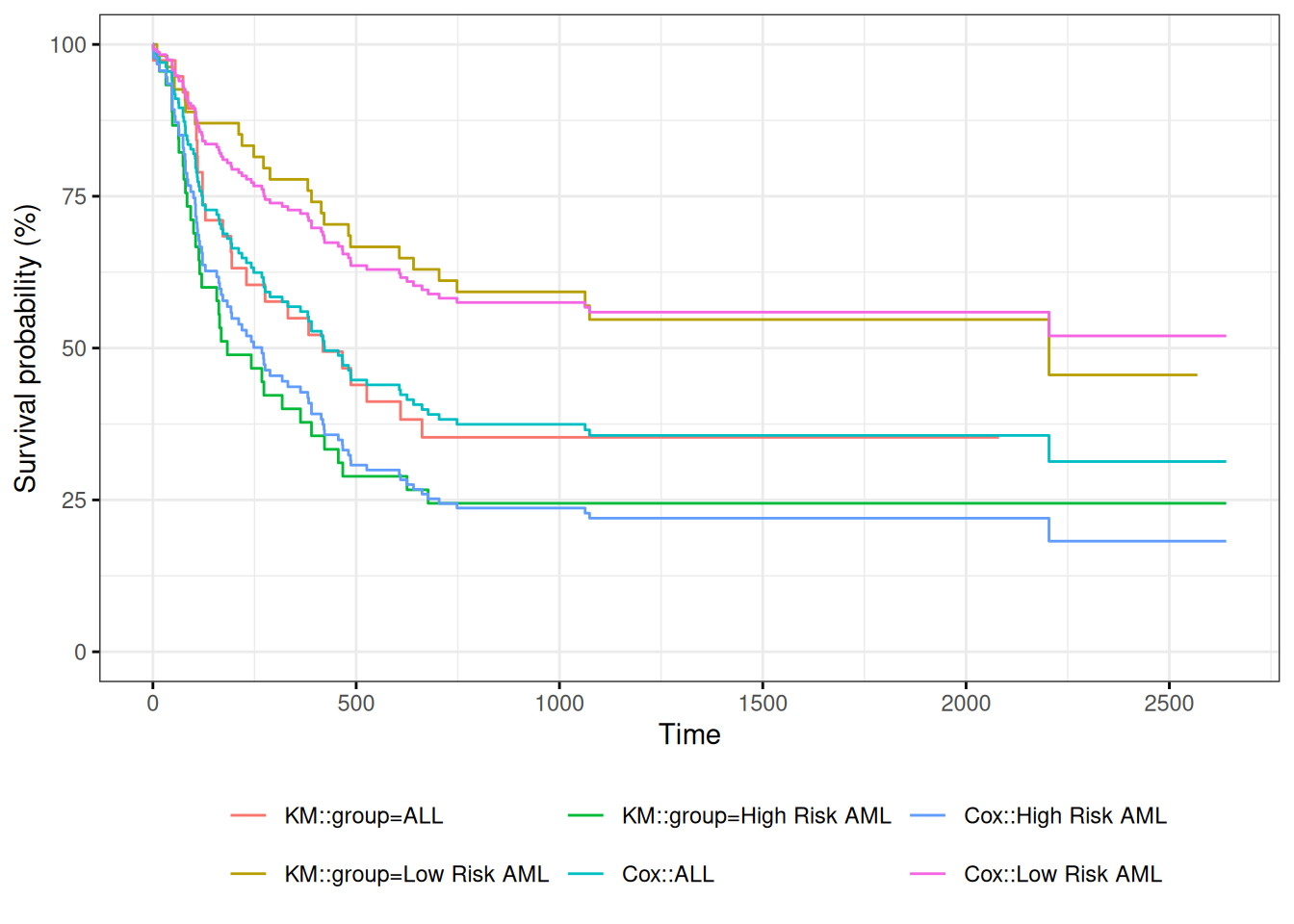
We can take a look at the resulting group-specific curves:

km_fit = survfit(Surv(t2, d3) ~ group, data = as.data.frame(bmt))

cox_fit = survfit(
  bmt.cox,
  newdata =
    data.frame(
      group = unique(bmt$group),
      row.names = unique(bmt$group)))

library(survminer)

list(KM = km_fit, Cox = cox_fit) |>
  survminer::ggsurvplot(
    # facet.by = "group",
    legend = "bottom",
    legend.title = "",
    combine = TRUE,
    fun = 'pct',
    size = .5,
    ggtheme = theme_bw(),
    conf.int = FALSE,
    censor = FALSE) |>
  suppressWarnings() # ggsurvplot() throws some warnings that aren't too worrying

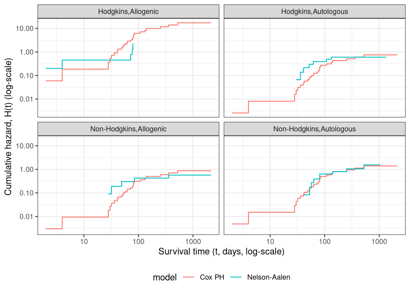
Figure 6: Survival Functions for Three Groups by KM and Cox Model

When we use survfit() with a Cox model, we have to specify the covariate levels we are interested in; the argument newdata should include a data.frame with the same named columns as the predictors in the Cox model and one or more levels of each.

From ?survfit.coxph:

If the newdata argument is missing, a curve is produced for a single “pseudo” subject with covariate values equal to the means component of the fit. The resulting curve(s) almost never make sense, but the default remains due to an unwarranted attachment to the option shown by some users and by other packages. Two particularly egregious examples are factor variables and interactions. Suppose one were studying interspecies transmission of a virus, and the data set has a factor variable with levels (“pig”, “chicken”) and about equal numbers of observations for each. The “mean” covariate level will be 0.5 – is this a flying pig?

Examining survfit

survfit(Surv(t2, d3) ~ group, data = bmt)
#> Call: survfit(formula = Surv(t2, d3) ~ group, data = bmt)
#> 
#>                      n events median 0.95LCL 0.95UCL
#> group=ALL           38     24    418     194      NA
#> group=Low Risk AML  54     25   2204     704      NA
#> group=High Risk AML 45     34    183     115     456

survfit(Surv(t2, d3) ~ group, data = bmt) |> summary()
#> Call: survfit(formula = Surv(t2, d3) ~ group, data = bmt)
#> 
#>                 group=ALL 
#>  time n.risk n.event survival std.err lower 95% CI upper 95% CI
#>     1     38       1    0.974  0.0260        0.924        1.000
#>    55     37       1    0.947  0.0362        0.879        1.000
#>    74     36       1    0.921  0.0437        0.839        1.000
#>    86     35       1    0.895  0.0498        0.802        0.998
#>   104     34       1    0.868  0.0548        0.767        0.983
#>   107     33       1    0.842  0.0592        0.734        0.966
#>   109     32       1    0.816  0.0629        0.701        0.949
#>   110     31       1    0.789  0.0661        0.670        0.930
#>   122     30       2    0.737  0.0714        0.609        0.891
#>   129     28       1    0.711  0.0736        0.580        0.870
#>   172     27       1    0.684  0.0754        0.551        0.849
#>   192     26       1    0.658  0.0770        0.523        0.827
#>   194     25       1    0.632  0.0783        0.495        0.805
#>   230     23       1    0.604  0.0795        0.467        0.782
#>   276     22       1    0.577  0.0805        0.439        0.758
#>   332     21       1    0.549  0.0812        0.411        0.734
#>   383     20       1    0.522  0.0817        0.384        0.709
#>   418     19       1    0.494  0.0819        0.357        0.684
#>   466     18       1    0.467  0.0818        0.331        0.658
#>   487     17       1    0.439  0.0815        0.305        0.632
#>   526     16       1    0.412  0.0809        0.280        0.605
#>   609     14       1    0.382  0.0803        0.254        0.577
#>   662     13       1    0.353  0.0793        0.227        0.548
#> 
#>                 group=Low Risk AML 
#>  time n.risk n.event survival std.err lower 95% CI upper 95% CI
#>    10     54       1    0.981  0.0183        0.946        1.000
#>    35     53       1    0.963  0.0257        0.914        1.000
#>    48     52       1    0.944  0.0312        0.885        1.000
#>    53     51       1    0.926  0.0356        0.859        0.998
#>    79     50       1    0.907  0.0394        0.833        0.988
#>    80     49       1    0.889  0.0428        0.809        0.977
#>   105     48       1    0.870  0.0457        0.785        0.965
#>   211     47       1    0.852  0.0483        0.762        0.952
#>   219     46       1    0.833  0.0507        0.740        0.939
#>   248     45       1    0.815  0.0529        0.718        0.925
#>   272     44       1    0.796  0.0548        0.696        0.911
#>   288     43       1    0.778  0.0566        0.674        0.897
#>   381     42       1    0.759  0.0582        0.653        0.882
#>   390     41       1    0.741  0.0596        0.633        0.867
#>   414     40       1    0.722  0.0610        0.612        0.852
#>   421     39       1    0.704  0.0621        0.592        0.837
#>   481     38       1    0.685  0.0632        0.572        0.821
#>   486     37       1    0.667  0.0642        0.552        0.805
#>   606     36       1    0.648  0.0650        0.533        0.789
#>   641     35       1    0.630  0.0657        0.513        0.773
#>   704     34       1    0.611  0.0663        0.494        0.756
#>   748     33       1    0.593  0.0669        0.475        0.739
#>  1063     26       1    0.570  0.0681        0.451        0.720
#>  1074     25       1    0.547  0.0691        0.427        0.701
#>  2204      6       1    0.456  0.1012        0.295        0.704
#> 
#>                 group=High Risk AML 
#>  time n.risk n.event survival std.err lower 95% CI upper 95% CI
#>     2     45       1    0.978  0.0220        0.936        1.000
#>    16     44       1    0.956  0.0307        0.897        1.000
#>    32     43       1    0.933  0.0372        0.863        1.000
#>    47     42       2    0.889  0.0468        0.802        0.986
#>    48     40       1    0.867  0.0507        0.773        0.972
#>    63     39       1    0.844  0.0540        0.745        0.957
#>    64     38       1    0.822  0.0570        0.718        0.942
#>    74     37       1    0.800  0.0596        0.691        0.926
#>    76     36       1    0.778  0.0620        0.665        0.909
#>    80     35       1    0.756  0.0641        0.640        0.892
#>    84     34       1    0.733  0.0659        0.615        0.875
#>    93     33       1    0.711  0.0676        0.590        0.857
#>   100     32       1    0.689  0.0690        0.566        0.838
#>   105     31       1    0.667  0.0703        0.542        0.820
#>   113     30       1    0.644  0.0714        0.519        0.801
#>   115     29       1    0.622  0.0723        0.496        0.781
#>   120     28       1    0.600  0.0730        0.473        0.762
#>   157     27       1    0.578  0.0736        0.450        0.742
#>   162     26       1    0.556  0.0741        0.428        0.721
#>   164     25       1    0.533  0.0744        0.406        0.701
#>   168     24       1    0.511  0.0745        0.384        0.680
#>   183     23       1    0.489  0.0745        0.363        0.659
#>   242     22       1    0.467  0.0744        0.341        0.638
#>   268     21       1    0.444  0.0741        0.321        0.616
#>   273     20       1    0.422  0.0736        0.300        0.594
#>   318     19       1    0.400  0.0730        0.280        0.572
#>   363     18       1    0.378  0.0723        0.260        0.550
#>   390     17       1    0.356  0.0714        0.240        0.527
#>   422     16       1    0.333  0.0703        0.221        0.504
#>   456     15       1    0.311  0.0690        0.201        0.481
#>   467     14       1    0.289  0.0676        0.183        0.457
#>   625     13       1    0.267  0.0659        0.164        0.433
#>   677     12       1    0.244  0.0641        0.146        0.409

survfit(bmt.cox)
#> Call: survfit(formula = bmt.cox)
#> 
#>        n events median 0.95LCL 0.95UCL
#> [1,] 137     83    422     268      NA
survfit(bmt.cox, newdata = tibble(group = unique(bmt$group)))
#> Call: survfit(formula = bmt.cox, newdata = tibble(group = unique(bmt$group)))
#> 
#>     n events median 0.95LCL 0.95UCL
#> 1 137     83    422     268      NA
#> 2 137     83     NA     625      NA
#> 3 137     83    268     162     467

bmt.cox |>
  survfit(newdata = tibble(group = unique(bmt$group))) |>
  summary()
#> Call: survfit(formula = bmt.cox, newdata = tibble(group = unique(bmt$group)))
#> 
#>  time n.risk n.event survival1 survival2 survival3
#>     1    137       1     0.993     0.996     0.989
#>     2    136       1     0.985     0.992     0.978
#>    10    135       1     0.978     0.987     0.968
#>    16    134       1     0.970     0.983     0.957
#>    32    133       1     0.963     0.979     0.946
#>    35    132       1     0.955     0.975     0.935
#>    47    131       2     0.941     0.966     0.914
#>    48    129       2     0.926     0.957     0.893
#>    53    127       1     0.918     0.953     0.882
#>    55    126       1     0.911     0.949     0.872
#>    63    125       1     0.903     0.944     0.861
#>    64    124       1     0.896     0.940     0.851
#>    74    123       2     0.881     0.931     0.830
#>    76    121       1     0.873     0.926     0.819
#>    79    120       1     0.865     0.922     0.809
#>    80    119       2     0.850     0.913     0.788
#>    84    117       1     0.843     0.908     0.778
#>    86    116       1     0.835     0.903     0.768
#>    93    115       1     0.827     0.899     0.757
#>   100    114       1     0.820     0.894     0.747
#>   104    113       1     0.812     0.889     0.737
#>   105    112       2     0.797     0.880     0.717
#>   107    110       1     0.789     0.875     0.707
#>   109    109       1     0.782     0.870     0.697
#>   110    108       1     0.774     0.866     0.687
#>   113    107       1     0.766     0.861     0.677
#>   115    106       1     0.759     0.856     0.667
#>   120    105       1     0.751     0.851     0.657
#>   122    104       2     0.735     0.841     0.637
#>   129    102       1     0.727     0.836     0.627
#>   157    101       1     0.720     0.831     0.617
#>   162    100       1     0.712     0.826     0.607
#>   164     99       1     0.704     0.821     0.598
#>   168     98       1     0.696     0.815     0.588
#>   172     97       1     0.688     0.810     0.578
#>   183     96       1     0.680     0.805     0.568
#>   192     95       1     0.672     0.800     0.558
#>   194     94       1     0.664     0.794     0.549
#>   211     93       1     0.656     0.789     0.539
#>   219     92       1     0.648     0.783     0.530
#>   230     90       1     0.640     0.778     0.520
#>   242     89       1     0.632     0.773     0.511
#>   248     88       1     0.624     0.767     0.501
#>   268     87       1     0.616     0.761     0.492
#>   272     86       1     0.608     0.756     0.482
#>   273     85       1     0.600     0.750     0.473
#>   276     84       1     0.592     0.745     0.464
#>   288     83       1     0.584     0.739     0.454
#>   318     82       1     0.576     0.733     0.445
#>   332     81       1     0.568     0.727     0.436
#>   363     80       1     0.560     0.722     0.427
#>   381     79       1     0.552     0.716     0.418
#>   383     78       1     0.544     0.710     0.409
#>   390     77       2     0.528     0.698     0.392
#>   414     75       1     0.520     0.692     0.383
#>   418     74       1     0.512     0.686     0.374
#>   421     73       1     0.504     0.680     0.366
#>   422     72       1     0.496     0.674     0.357
#>   456     71       1     0.488     0.667     0.349
#>   466     70       1     0.480     0.661     0.340
#>   467     69       1     0.472     0.655     0.332
#>   481     68       1     0.464     0.649     0.324
#>   486     67       1     0.455     0.642     0.315
#>   487     66       1     0.447     0.636     0.307
#>   526     65       1     0.439     0.629     0.299
#>   606     63       1     0.431     0.623     0.291
#>   609     62       1     0.423     0.616     0.283
#>   625     61       1     0.415     0.609     0.275
#>   641     60       1     0.407     0.603     0.267
#>   662     59       1     0.399     0.596     0.260
#>   677     58       1     0.391     0.589     0.252
#>   704     57       1     0.383     0.582     0.244
#>   748     56       1     0.374     0.575     0.237
#>  1063     47       1     0.365     0.567     0.228
#>  1074     46       1     0.356     0.559     0.220
#>  2204      9       1     0.313     0.520     0.182

6 Adjustment for Ties (optional)

At each time \(t_i\) at which more than one of the subjects has an event, let \(d_i\) be the number of events at that time, \(D_i\) the set of subjects with events at that time, and let \(s_i\) be a covariate vector for an artificial subject obtained by adding up the covariate values for the subjects with an event at time \(t_i\). Let \[\bar\eta_i = \beta_1s_{i1}+\cdots+\beta_ps_{ip}\] and \(\bar\theta_i = \text{exp}{\left\{\bar\eta_i\right\}}\).

Let \(s_i\) be a covariate vector for an artificial subject obtained by adding up the covariate values for the subjects with an event at time \(t_i\). Note that

\[ \begin{aligned} \bar\eta_i &=\sum_{j \in D_i}\beta_1x_{j1}+\cdots+\beta_px_{jp}\\ &= \beta_1s_{i1}+\cdots+\beta_ps_{ip}\\ \bar\theta_i &= \text{exp}{\left\{\bar\eta_i\right\}}\\ &= \prod_{j \in D_i}\theta_i \end{aligned} \]

Breslow’s method for ties

Breslow’s method estimates the partial likelihood as

\[ \begin{aligned} L(\beta|T) &= \prod_i \frac{\bar\theta_i}{[\sum_{k \in R(t_i)} \theta_k]^{d_i}}\\ &= \prod_i \prod_{j \in D_i}\frac{\theta_j}{\sum_{k \in R(t_i)} \theta_k} \end{aligned} \]

This method is equivalent to treating each event as distinct and using the non-ties formula. It works best when the number of ties is small. It is the default in many statistical packages, including PROC PHREG in SAS.

Efron’s method for ties

The other common method is Efron’s, which is the default in R.

\[L(\beta|T)= \prod_i \frac{\bar\theta_i}{\prod_{j=1}^{d_i}[\sum_{k \in R(t_i)} \theta_k-\frac{j-1}{d_i}\sum_{k \in D_i} \theta_k]}\] This is closer to the exact discrete partial likelihood when there are many ties.

The third option in R (and an option also in SAS as discrete) is the “exact” method, which is the same one used for matched logistic regression.

Example: Breslow’s method

Suppose as an example we have a time \(t\) where there are 20 individuals at risk and three failures. Let the three individuals have risk parameters \(\theta_1, \theta_2, \theta_3\) and let the sum of the risk parameters of the remaining 17 individuals be \(\theta_R\). Then the factor in the partial likelihood at time \(t\) using Breslow’s method is

\[ \left(\frac{\theta_1}{\theta_R+\theta_1+\theta_2+\theta_3}\right) \left(\frac{\theta_2}{\theta_R+\theta_1+\theta_2+\theta_3}\right) \left(\frac{\theta_3}{\theta_R+\theta_1+\theta_2+\theta_3}\right) \]

If on the other hand, they had died in the order 1,2, 3, then the contribution to the partial likelihood would be:

\[ \left(\frac{\theta_1}{\theta_R+\theta_1+\theta_2+\theta_3}\right) \left(\frac{\theta_2}{\theta_R+\theta_2+\theta_3}\right) \left(\frac{\theta_3}{\theta_R+\theta_3}\right) \]

as the risk set got smaller with each failure. The exact method roughly averages the results for the six possible orderings of the failures.

Example: Efron’s method

But we don’t know the order they failed in, so instead of reducing the denominator by one risk coefficient each time, we reduce it by the same fraction. This is Efron’s method.

\[\left(\frac{\theta_1}{\theta_R+\theta_1+\theta_2+\theta_3}\right) \left(\frac{\theta_2}{\theta_R+2(\theta_1+\theta_2+\theta_3)/3}\right) \left(\frac{\theta_3}{\theta_R+(\theta_1+\theta_2+\theta_3)/3}\right)\]

6.1 Building Cox Proportional Hazards models

hodg Lymphoma Data Set from KMsurv

Participants

43 bone marrow transplant patients at Ohio State University (Avalos 1993)

Variables

• dtype: Disease type (Hodgkin’s or non-Hodgkins lymphoma)
• gtype: Bone marrow graft type:
• allogeneic: from HLA-matched sibling
• autologous: from self (prior to chemo)
• time: time to study exit
• delta: study exit reason (death/relapse vs censored)
• wtime: waiting time to transplant (in months)
• score: Karnofsky score:
• 80–100: Able to carry on normal activity and to work; no special care needed.
• 50–70: Unable to work; able to live at home and care for most personal needs; varying amount of assistance needed.
• 10–60: Unable to care for self; requires equivalent of institutional or hospital care; disease may be progressing rapidly.

Data

library(dplyr)
library(survival)
data(hodg, package = "KMsurv")
hodg2 = hodg |> 
  as_tibble() |> 
  mutate(
    # We add factor labels to the categorical variables:
    gtype = gtype |> 
      case_match(
        1 ~ "Allogenic",
        2 ~ "Autologous"),
    dtype = dtype |> 
      case_match(
        1 ~ "Non-Hodgkins",
        2 ~ "Hodgkins") |> 
      factor() |> 
      relevel(ref = "Non-Hodgkins"), 
    delta = delta |> 
      case_match(
        1 ~ "dead",
        0 ~ "alive"),
    surv = Surv(
      time = time, 
      event = delta == "dead")
  )
hodg2 |> print()
#> # A tibble: 43 × 7
#>    gtype     dtype         time delta score wtime   surv
#>    <chr>     <fct>        <int> <chr> <int> <int> <Surv>
#>  1 Allogenic Non-Hodgkins    28 dead     90    24    28 
#>  2 Allogenic Non-Hodgkins    32 dead     30     7    32 
#>  3 Allogenic Non-Hodgkins    49 dead     40     8    49 
#>  4 Allogenic Non-Hodgkins    84 dead     60    10    84 
#>  5 Allogenic Non-Hodgkins   357 dead     70    42   357 
#>  6 Allogenic Non-Hodgkins   933 alive    90     9   933+
#>  7 Allogenic Non-Hodgkins  1078 alive   100    16  1078+
#>  8 Allogenic Non-Hodgkins  1183 alive    90    16  1183+
#>  9 Allogenic Non-Hodgkins  1560 alive    80    20  1560+
#> 10 Allogenic Non-Hodgkins  2114 alive    80    27  2114+
#> # ℹ 33 more rows

Proportional hazards model

Table 1: Summary of Proportional Hazards model for Hodgkins Lymphoma data

hodg.cox1 = coxph(
  formula = surv ~ gtype * dtype + score + wtime, 
  data = hodg2)

summary(hodg.cox1)
#> Call:
#> coxph(formula = surv ~ gtype * dtype + score + wtime, data = hodg2)
#> 
#>   n= 43, number of events= 26 
#> 
#>                                  coef exp(coef) se(coef)     z Pr(>|z|)    
#> gtypeAutologous                0.6394    1.8953   0.5937  1.08   0.2815    
#> dtypeHodgkins                  2.7603   15.8050   0.9474  2.91   0.0036 ** 
#> score                         -0.0495    0.9517   0.0124 -3.98  6.8e-05 ***
#> wtime                         -0.0166    0.9836   0.0102 -1.62   0.1046    
#> gtypeAutologous:dtypeHodgkins -2.3709    0.0934   1.0355 -2.29   0.0220 *  
#> ---
#> Signif. codes:  0 '***' 0.001 '**' 0.01 '*' 0.05 '.' 0.1 ' ' 1
#> 
#>                               exp(coef) exp(-coef) lower .95 upper .95
#> gtypeAutologous                  1.8953     0.5276    0.5920     6.068
#> dtypeHodgkins                   15.8050     0.0633    2.4682   101.207
#> score                            0.9517     1.0507    0.9288     0.975
#> wtime                            0.9836     1.0167    0.9641     1.003
#> gtypeAutologous:dtypeHodgkins    0.0934    10.7074    0.0123     0.711
#> 
#> Concordance= 0.776  (se = 0.059 )
#> Likelihood ratio test= 32.1  on 5 df,   p=6e-06
#> Wald test            = 27.2  on 5 df,   p=5e-05
#> Score (logrank) test = 37.7  on 5 df,   p=4e-07

6.2 Diagnostic graphs for proportional hazards assumption

Analysis plan

• survival function for the four combinations of disease type and graft type.
• observed (nonparametric) vs. expected (semiparametric) survival functions.
• complementary log-log survival for the four groups.

Kaplan-Meier survival functions

km_model = survfit(
  formula = surv ~ dtype + gtype,
  data = hodg2)

library(ggplot2)
km_model |> 
  autoplot(conf.int = FALSE) +
  theme_bw() +
  theme(
    legend.position="bottom",
    legend.title = element_blank(),
    legend.text = element_text(size = legend_text_size)
  ) +
  guides(col=guide_legend(ncol=2)) +
  ylab('Survival probability, S(t)') +
  xlab("Time since transplant (days)")

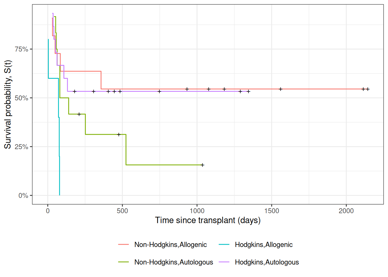
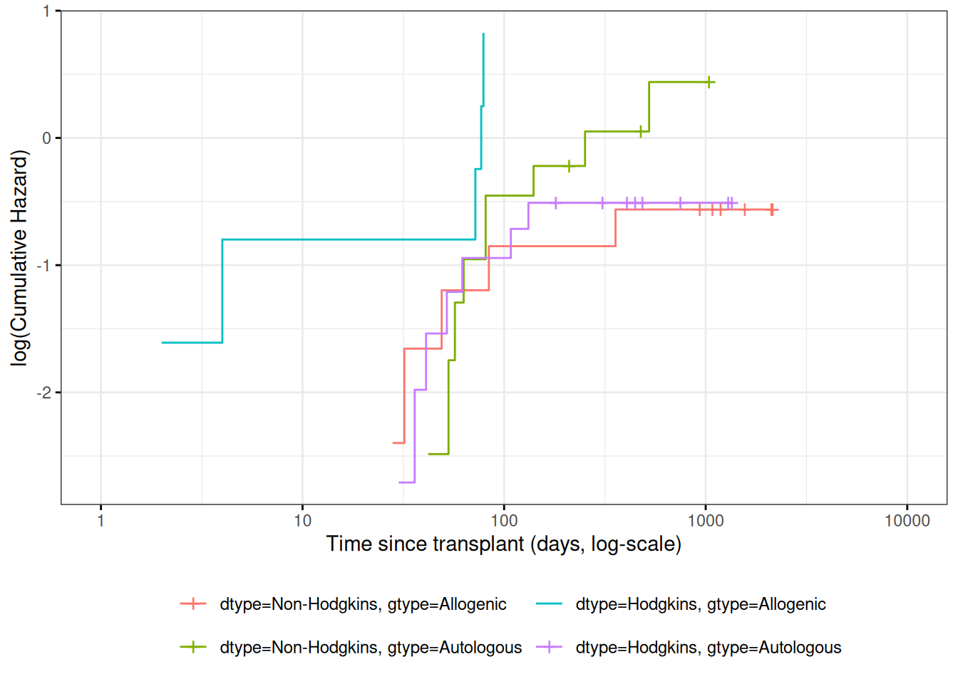
Figure 7: Kaplan-Meier Survival Curves for HOD/NHL and Allo/Auto Grafts

Observed and expected survival curves

# we need to create a tibble of covariate patterns;
# we will set score and wtime to mean values for disease and graft types:
means = hodg2 |> 
  summarize(
    .by = c(dtype, gtype), 
    score = mean(score), 
    wtime = mean(wtime)) |> 
  arrange(dtype, gtype) |> 
  mutate(strata = paste(dtype, gtype, sep = ",")) |> 
  as.data.frame() 

# survfit.coxph() will use the rownames of its `newdata`
# argument to label its output:
rownames(means) = means$strata

cox_model = 
  hodg.cox1 |> 
  survfit(
    data = hodg2, # ggsurvplot() will need this
    newdata = means)

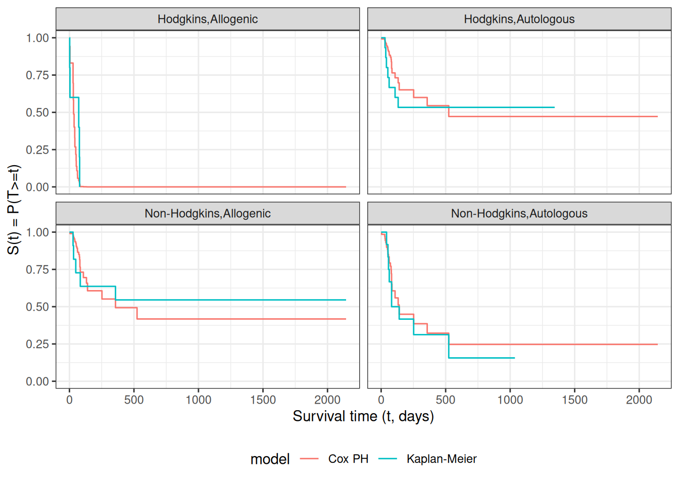
# I couldn't find a good function to reformat `cox_model` for ggplot, 
# so I made my own:
stack_surv_ph = function(cox_model)
{
  cox_model$surv |> 
    as_tibble() |> 
    mutate(time = cox_model$time) |> 
    pivot_longer(
      cols = -time,
      names_to = "strata",
      values_to = "surv") |> 
    mutate(
      cumhaz = -log(surv),
      model = "Cox PH")
}

km_and_cph =
  km_model |> 
  fortify(surv.connect = TRUE) |> 
  mutate(
    strata = trimws(strata),
    model = "Kaplan-Meier",
    cumhaz = -log(surv)) |>
  bind_rows(stack_surv_ph(cox_model))

km_and_cph |> 
  ggplot(aes(x = time, y = surv, col = model)) +
  geom_step() +
  facet_wrap(~strata) +
  theme_bw() + 
  ylab("S(t) = P(T>=t)") +
  xlab("Survival time (t, days)") +
  theme(legend.position = "bottom")

Observed and expected survival curves for bmt data

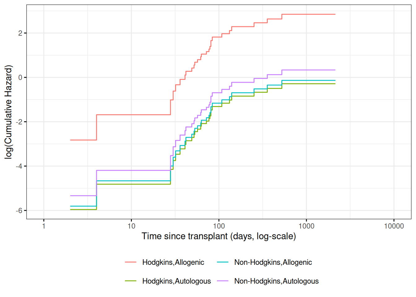
Cumulative hazard (log-scale) curves

Also known as “complementary log-log (clog-log) survival curves”.

na_model = survfit(
  formula = surv ~ dtype + gtype,
  data = hodg2,
  type = "fleming")

na_model |> 
  survminer::ggsurvplot(
  legend = "bottom", 
  legend.title = "",
  ylab = "log(Cumulative Hazard)",
  xlab = "Time since transplant (days, log-scale)",
  fun = 'cloglog', 
  size = .5,
  ggtheme = theme_bw(),
  conf.int = FALSE, 
  censor = TRUE) |>  
  magrittr::extract2("plot") +
  guides(
    col = 
      guide_legend(
        ncol = 2,
        label.theme = 
          element_text(
            size = legend_text_size)))

Figure 8: Complementary log-log survival curves - Nelson-Aalen estimates

Let’s compare these empirical (i.e., non-parametric) curves with the fitted curves from our coxph() model:

cox_model |> 
  survminer::ggsurvplot(
    facet_by = "",
    legend = "bottom", 
    legend.title = "",
    ylab = "log(Cumulative Hazard)",
    xlab = "Time since transplant (days, log-scale)",
    fun = 'cloglog', 
    size = .5,
    ggtheme = theme_bw(),
    censor = FALSE, # doesn't make sense for cox model
    conf.int = FALSE) |>  
  magrittr::extract2("plot") +
  guides(
    col = 
      guide_legend(
        ncol = 2,
        label.theme = 
          element_text(
            size = legend_text_size)))

Figure 9: Complementary log-log survival curves - PH estimates

Now let’s overlay these cumulative hazard curves:

na_and_cph = 
  na_model |> 
  fortify(fun = "cumhaz") |> 
  # `fortify.survfit()` doesn't name cumhaz correctly:
  rename(cumhaz = surv) |>  
  mutate(
    surv = exp(-cumhaz),
    strata = trimws(strata)) |> 
  mutate(model = "Nelson-Aalen") |> 
  bind_rows(stack_surv_ph(cox_model))

na_and_cph |> 
  ggplot(
    aes(
      x = time, 
      y = cumhaz, 
      col = model)) +
  geom_step() +
  facet_wrap(~strata) +
  theme_bw() + 
  scale_y_continuous(
    trans = "log10",
    name = "Cumulative hazard, H(t) (log-scale)") +
  scale_x_continuous(
    trans = "log10",
    name = "Survival time (t, days, log-scale)") +
  theme(legend.position = "bottom")

Figure 10: Observed and expected cumulative hazard curves for bmt data (cloglog format)

6.3 Predictions and Residuals

Review: Predictions in Linear Regression

• In linear regression, we have a linear predictor for each data point \(i\)

\[ \begin{aligned} \eta_i &= \beta_0+\beta_1x_{1i}+\cdots+\beta_px_{pi}\\ \hat y_i &=\hat\eta_i = \hat\beta_0+\hat\beta_1x_{1i}+\cdots+\hat\beta_px_{pi}\\ y_i &\sim N(\eta_i,\sigma^2) \end{aligned} \]

• \(\hat y_i\) estimates the conditional mean of \(y_i\) given the covariate values \(\tilde{x}_i\). This together with the prediction error says that we are predicting the distribution of values of \(y\).

Review: Residuals in Linear Regression

• The usual residual is \(r_i=y_i-\hat y_i\), the difference between the actual value of \(y\) and a prediction of its mean.
• The residuals are also the quantities the sum of whose squares is being minimized by the least squares/MLE estimation.

Predictions and Residuals in survival models

• In survival analysis, the equivalent of \(y_i\) is the event time \(t_i\), which is unknown for the censored observations.
• The expected event time can be tricky to calculate:

\[ \hat{\text{E}}[T|X=x] = \int_{t=0}^{\infty} \hat{\text{S}}(t)dt \]

Wide prediction intervals

The nature of time-to-event data results in very wide prediction intervals:

• Suppose a cancer patient is predicted to have a mean lifetime of 5 years after diagnosis and suppose the distribution is exponential.
• If we want a 95% interval for survival, the lower end is at the 0.025 percentage point of the exponential which is qexp(.025, rate = 1/5) = 0.126589 years, or 1/40 of the mean lifetime.
• The upper end is at the 0.975 point which is qexp(.975, rate = 1/5) = 18.444397 years, or 3.7 times the mean lifetime.
• Saying that the survival time is somewhere between 6 weeks and 18 years does not seem very useful, but it may be the best we can do.
• For survival analysis, something is like a residual if it is small when the model is accurate or if the accumulation of them is in some way minimized by the estimation algorithm, but there is no exact equivalence to linear regression residuals.
• And if there is, they are mostly quite large!

Types of Residuals in Time-to-Event Models

• It is often hard to make a decision from graph appearances, though the process can reveal much.
• Some diagnostic tests are based on residuals as with other regression methods:
  • Schoenfeld residuals (via cox.zph) for proportionality
  • Cox-Snell residuals for goodness of fit (Section 6.4)
  • martingale residuals for non-linearity
  • dfbeta for influence.

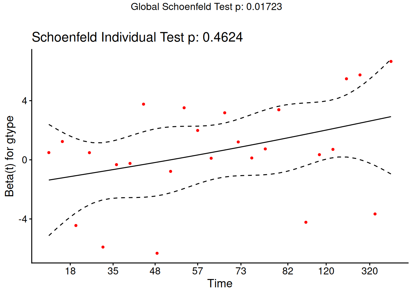
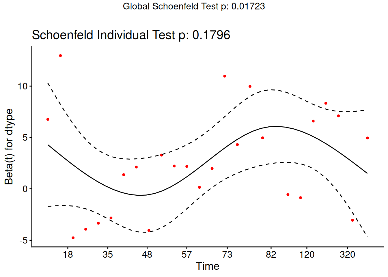
Schoenfeld residuals

• There is a Schoenfeld residual for each subject \(i\) with an event (not censored) and for each predictor \(x_{k}\).

• At the event time \(t\) for that subject, there is a risk set \(R\), and each subject \(j\) in the risk set has a risk coefficient \(\theta_j\) and also a value \(x_{jk}\) of the predictor.

• The Schoenfeld residual is the difference between \(x_{ik}\) and the risk-weighted average of all the \(x_{jk}\) over the risk set.

\[ r^S_{ik} = x_{ik}-\frac{\sum_{k\in R}x_{jk}\theta_k}{\sum_{k\in R}\theta_k} \]

This residual measures how typical the individual subject is with respect to the covariate at the time of the event. Since subjects should fail more or less uniformly according to risk, the Schoenfeld residuals should be approximately level over time, not increasing or decreasing.

We can test this with the correlation with time on some scale, which could be the time itself, the log time, or the rank in the set of failure times.

The default is to use the KM curve as a transform, which is similar to the rank but deals better with censoring.

The cox.zph() function implements a score test proposed in Grambsch and Therneau (1994).

hodg.zph = cox.zph(hodg.cox1)
print(hodg.zph)
#>               chisq df     p
#> gtype        0.5400  1 0.462
#> dtype        1.8012  1 0.180
#> score        3.8805  1 0.049
#> wtime        0.0173  1 0.895
#> gtype:dtype  4.0474  1 0.044
#> GLOBAL      13.7573  5 0.017

gtype

ggcoxzph(hodg.zph, var = "gtype")

dtype

ggcoxzph(hodg.zph, var = "dtype")

score

ggcoxzph(hodg.zph, var = "score")

wtime

ggcoxzph(hodg.zph, var = "wtime")

gtype:dtype

ggcoxzph(hodg.zph, var = "gtype:dtype")

Conclusions

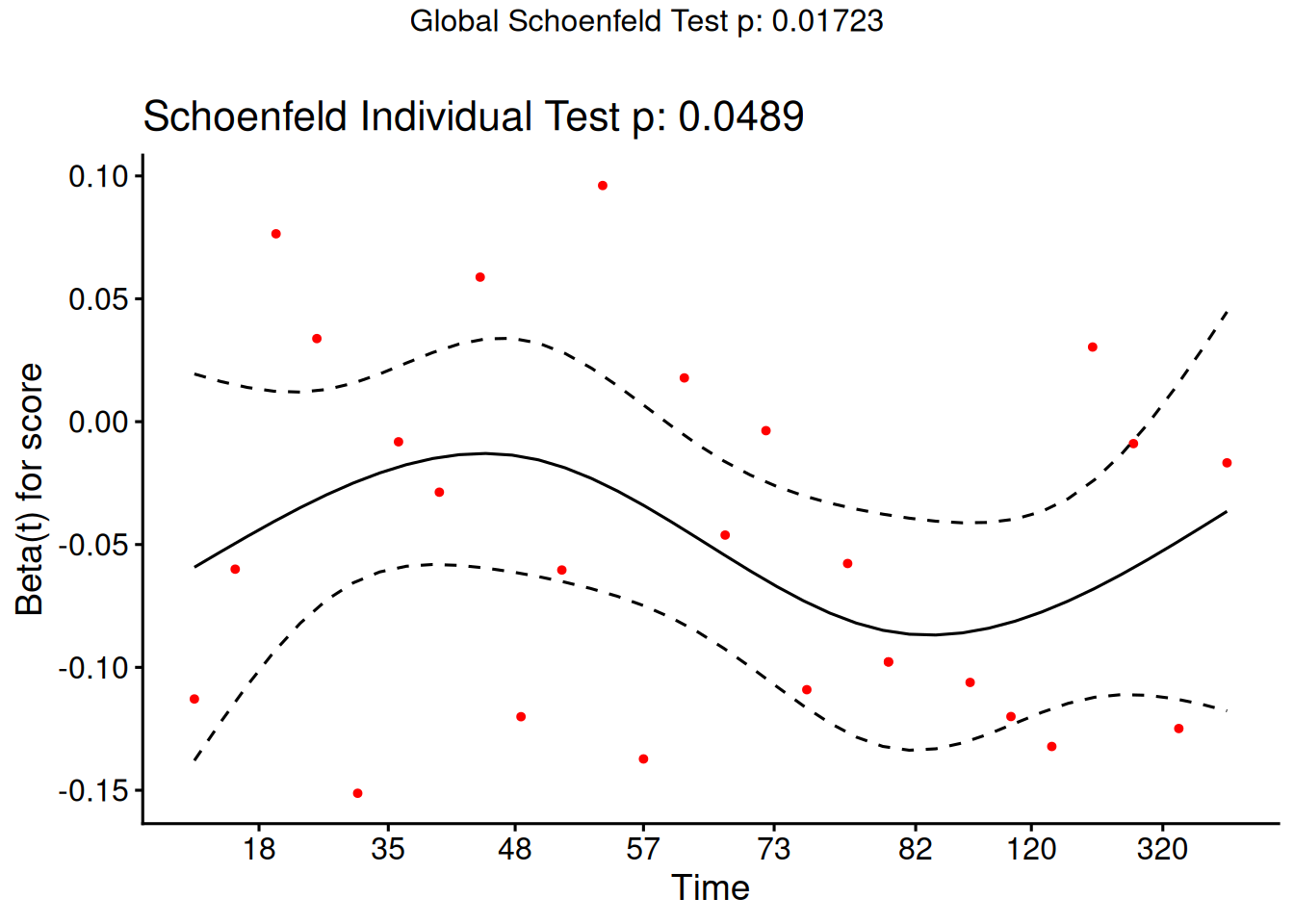
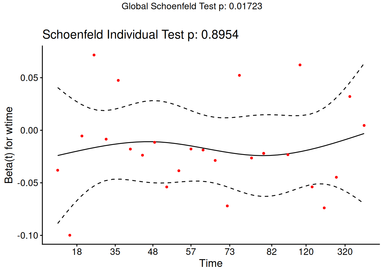
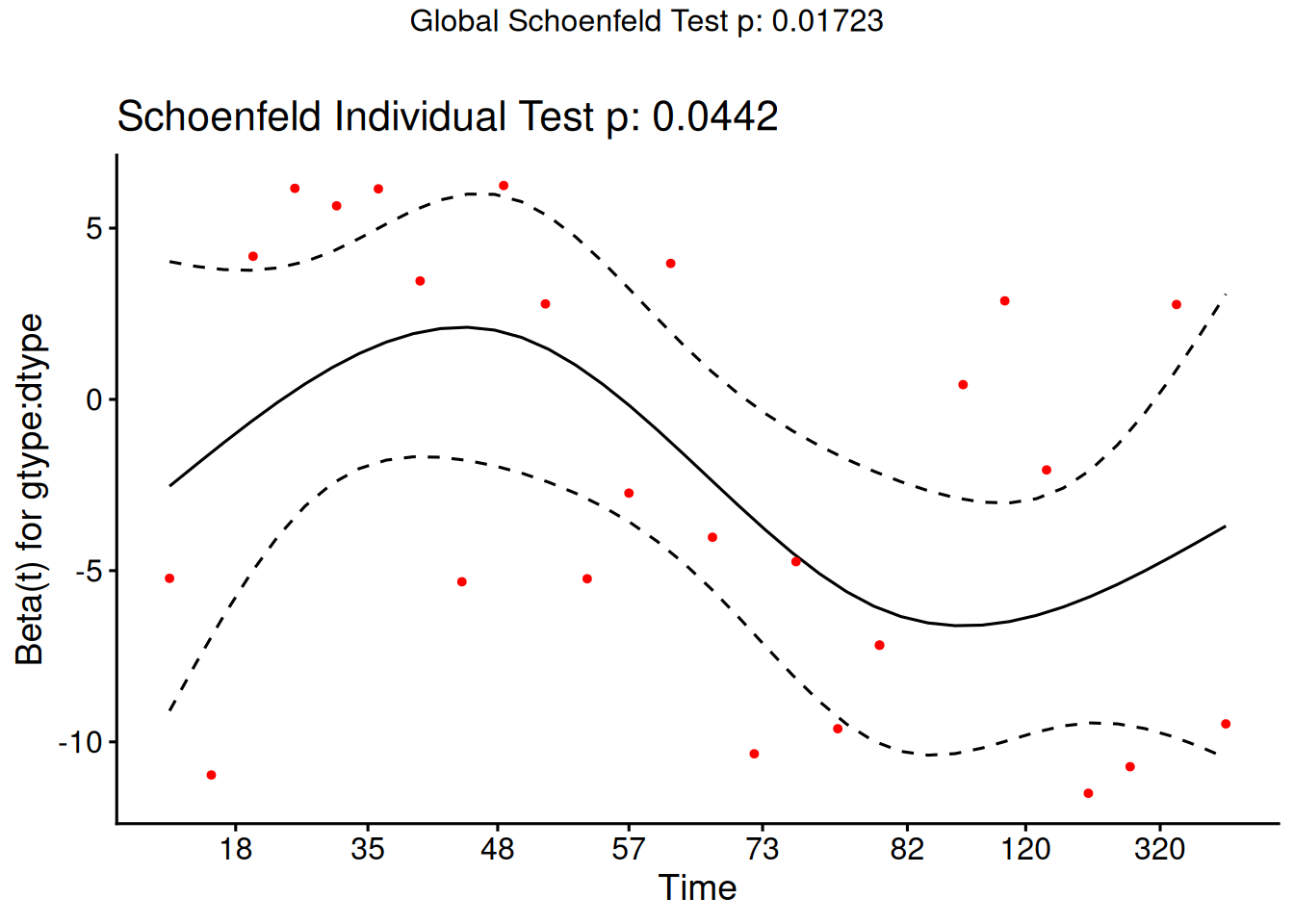
• From the correlation test, the Karnofsky score and the interaction with graft type disease type induce modest but statistically significant non-proportionality.
• The sample size here is relatively small (26 events in 43 subjects). If the sample size is large, very small amounts of non-proportionality can induce a significant result.
• As time goes on, autologous grafts are over-represented at their own event times, but those from HOD patients become less represented.
• Both the statistical tests and the plots are useful.

6.4 Goodness of Fit using the Cox-Snell Residuals

(references: Klein and Moeschberger (2003), §11.2, and Dobson and Barnett (2018), §10.6)

Suppose that an individual has a survival time \(T\) which has survival function \(\text{S}(t)\), meaning that \(\Pr(T> t) = \text{S}(t)\). Then \(S(T)\) has a uniform distribution on \((0,1)\):

\[ \begin{aligned} \Pr(S(T_i) \le u) &= \Pr(T_i > S_i^{-1}(u))\\ &= S_i(S_i^{-1}(u))\\ &= u \end{aligned} \]

Also, if \(U\) has a uniform distribution on \((0,1)\), then what is the distribution of \(-\ln(U)\)?

\[ \begin{aligned} \Pr(-\ln(U) < x) &= \Pr(U>\text{exp}{\left\{-x\right\}})\\ &= 1-e^{-x} \end{aligned} \]

which is the CDF of an exponential distribution with parameter \(\lambda=1\).

Definition 13 (Cox-Snell generalized residuals)  

The Cox-Snell generalized residuals are defined as:

\[ r^{CS}_i \stackrel{\text{def}}{=}\hat {\Lambda}(t_i|\tilde{x}_i) \]

If the estimate \(\hat S_i\) is accurate, \(r^{CS}_i\) should have an exponential distribution with constant hazard \(\lambda=1\), which means that these values should look like a censored sample from this exponential distribution.

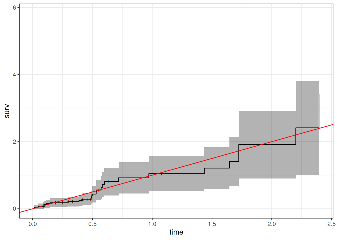
hodg2 = hodg2 |> 
  mutate(cs = predict(hodg.cox1, type = "expected"))

surv.csr = survfit(
  data = hodg2,
  formula = Surv(time = cs, event = delta == "dead") ~ 1,
  type = "fleming-harrington")

autoplot(surv.csr, fun = "cumhaz") + 
  geom_abline(aes(intercept = 0, slope = 1), col = "red") +
  theme_bw()

Figure 11: Cumulative Hazard of Cox-Snell Residuals

The line with slope 1 and intercept 0 fits the curve relatively well, so we don’t see lack of fit using this procedure.

6.5 Martingale Residuals

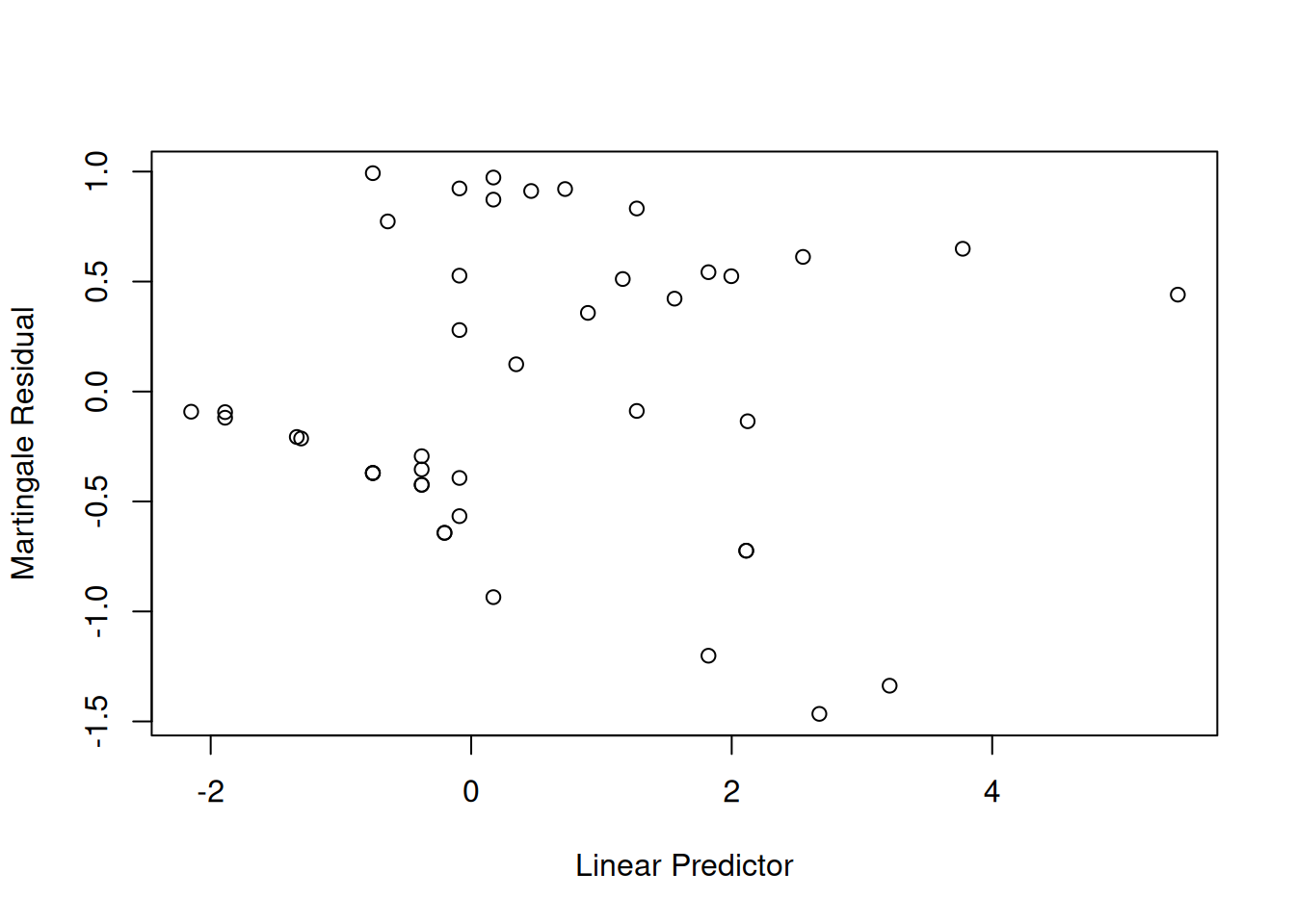
The martingale residuals are a slight modification of the Cox-Snell residuals. If the censoring indicator is \(\delta_i\), then \[r^M_i=\delta_i-r^{CS}_i\] These residuals can be interpreted as an estimate of the excess number of events seen in the data but not predicted by the model. We will use these to examine the functional forms of continuous covariates.

Using Martingale Residuals

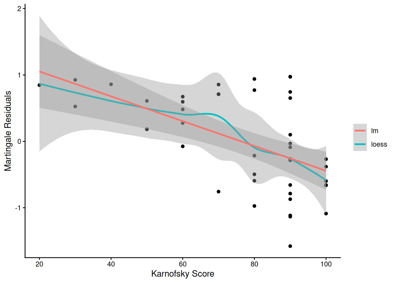
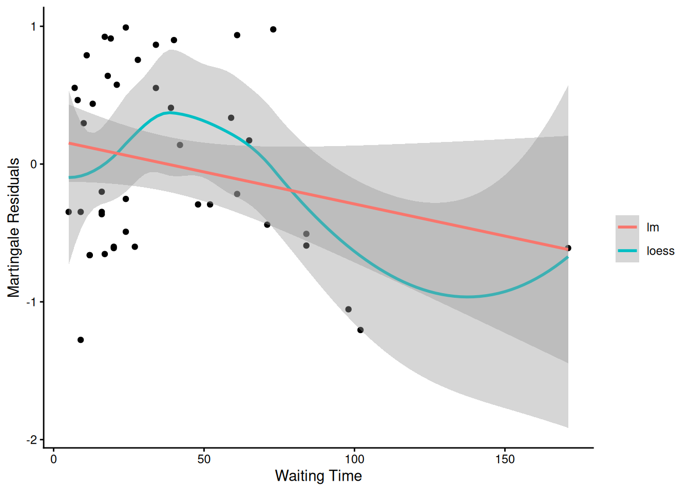
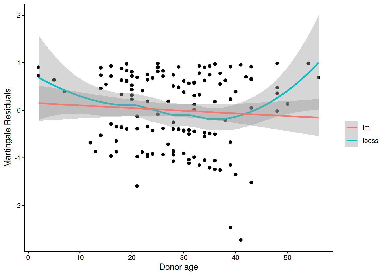
Martingale residuals can be used to examine the functional form of a numeric variable.

• We fit the model without that variable and compute the martingale residuals.
• We then plot these martingale residuals against the values of the variable.
• We can see curvature, or a possible suggestion that the variable can be discretized.

Let’s use this to examine the score and wtime variables in the wtime data set.

Karnofsky score

hodg2 = hodg2 |> 
  mutate(
    mres = 
      hodg.cox1 |> 
      update(. ~ . - score) |> 
      residuals(type="martingale"))

hodg2 |> 
  ggplot(aes(x = score, y = mres)) +
  geom_point() +
  geom_smooth(method = "loess", aes(col = "loess")) +
  geom_smooth(method = 'lm', aes(col = "lm")) +
  theme_classic() +
  xlab("Karnofsky Score") +
  ylab("Martingale Residuals") +
  guides(col=guide_legend(title = ""))

Martingale Residuals vs. Karnofsky Score

The line is almost straight. It could be some modest transformation of the Karnofsky score would help, but it might not make much difference.

Waiting time

hodg2$mres = 
  hodg.cox1 |> 
  update(. ~ . - wtime) |> 
  residuals(type="martingale")

hodg2 |> 
  ggplot(aes(x = wtime, y = mres)) +
  geom_point() +
  geom_smooth(method = "loess", aes(col = "loess")) +
  geom_smooth(method = 'lm', aes(col = "lm")) +
  theme_classic() +
  xlab("Waiting Time") +
  ylab("Martingale Residuals") +
  guides(col=guide_legend(title = ""))

Martingale Residuals vs. Waiting Time

The line could suggest a step function. To see where the drop is, we can look at the largest waiting times and the associated martingale residual.

The martingale residuals are all negative for wtime >83 and positive for the next smallest value. A reasonable cut-point is 80 days.

Updating the model

Let’s reformulate the model with dichotomized wtime.

hodg2 = 
  hodg2 |> 
  mutate(
    wt2 = cut(
      wtime,c(0, 80, 200),
      labels=c("short","long")))

hodg.cox2 =
  coxph(
    formula = 
      Surv(time, event = delta == "dead") ~ 
      gtype*dtype + score + wt2,
    data = hodg2)

hodg.cox1 |> drop1(test="Chisq")

Model summary table with waiting time on continuous scale

hodg.cox2 |> drop1(test="Chisq")

Model summary table with dichotomized waiting time

The new model has better (lower) AIC.

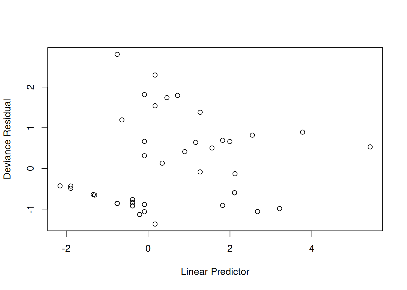
6.6 Checking for Outliers and Influential Observations

We will check for outliers using the deviance residuals. The martingale residuals show excess events or the opposite, but highly skewed, with the maximum possible value being 1, but the smallest value can be very large negative. Martingale residuals can detect unexpectedly long-lived patients, but patients who die unexpectedly early show up only in the deviance residual. Influence will be examined using dfbeta in a similar way to linear regression, logistic regression, or Poisson regression.

Deviance Residuals

\[ \begin{aligned} r_i^D &= \textrm{sign}(r_i^M)\sqrt{-2\left[ r_i^M+\delta_i\ln(\delta_i-r_i^M) \right]}\\ r_i^D &= \textrm{sign}(r_i^M)\sqrt{-2\left[ r_i^M+\delta_i\ln(r_i^{CS}) \right]} \end{aligned} \]

Roughly centered on 0 with approximate standard deviation 1.

hodg.mart = residuals(hodg.cox2,type="martingale")
hodg.dev = residuals(hodg.cox2,type="deviance")
hodg.dfb = residuals(hodg.cox2,type="dfbeta")
hodg.preds = predict(hodg.cox2)                   #linear predictor

plot(hodg.preds,
     hodg.mart,
     xlab="Linear Predictor",
     ylab="Martingale Residual")

Martingale Residuals vs. Linear Predictor

The smallest three martingale residuals in order are observations 1, 29, and 18.

plot(hodg.preds,hodg.dev,xlab="Linear Predictor",ylab="Deviance Residual")

Deviance Residuals vs. Linear Predictor

The two largest deviance residuals are observations 1 and 29. Worth examining.

dfbeta

• dfbeta is the approximate change in the coefficient vector if that observation were dropped

• dfbetas is the approximate change in the coefficients, scaled by the standard error for the coefficients.

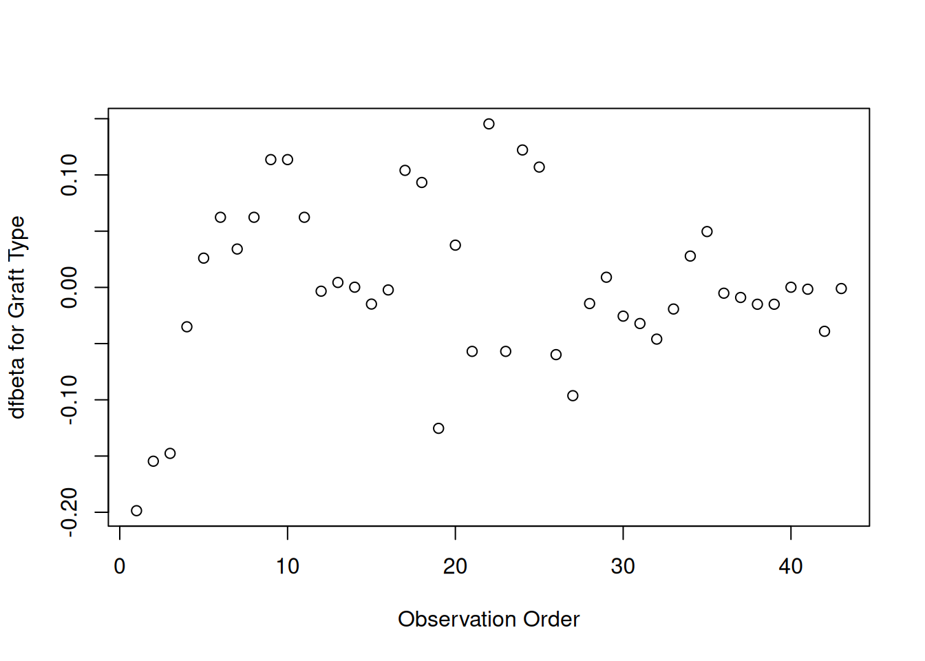
Graft type

plot(hodg.dfb[,1],xlab="Observation Order",ylab="dfbeta for Graft Type")

dfbeta Values by Observation Order for Graft Type

The smallest dfbeta for graft type is observation 1.

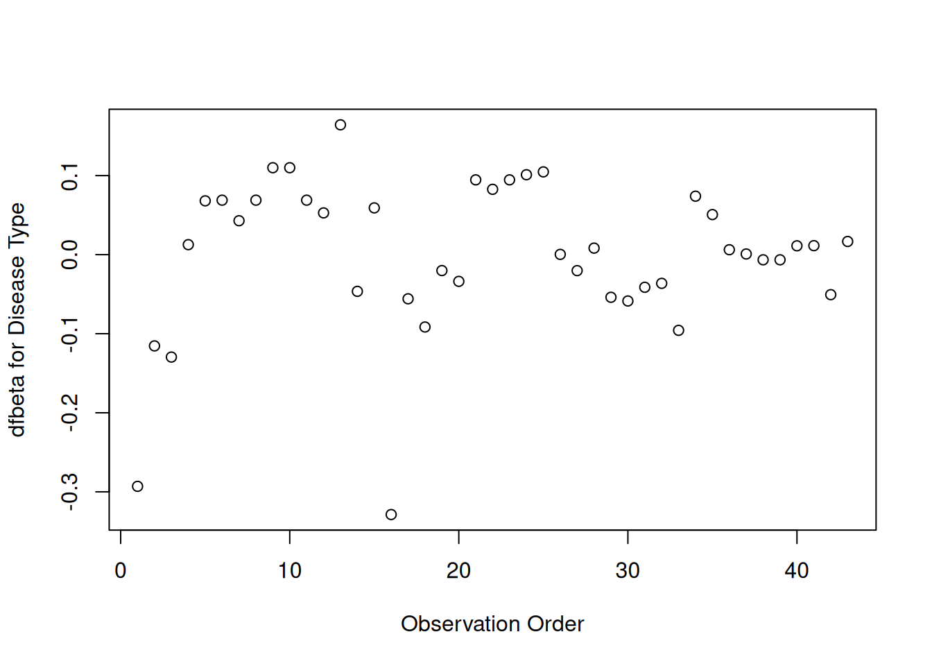
Disease type

plot(hodg.dfb[,2],
     xlab="Observation Order",
     ylab="dfbeta for Disease Type")

dfbeta Values by Observation Order for Disease Type

The smallest two dfbeta values for disease type are observations 1 and 16.

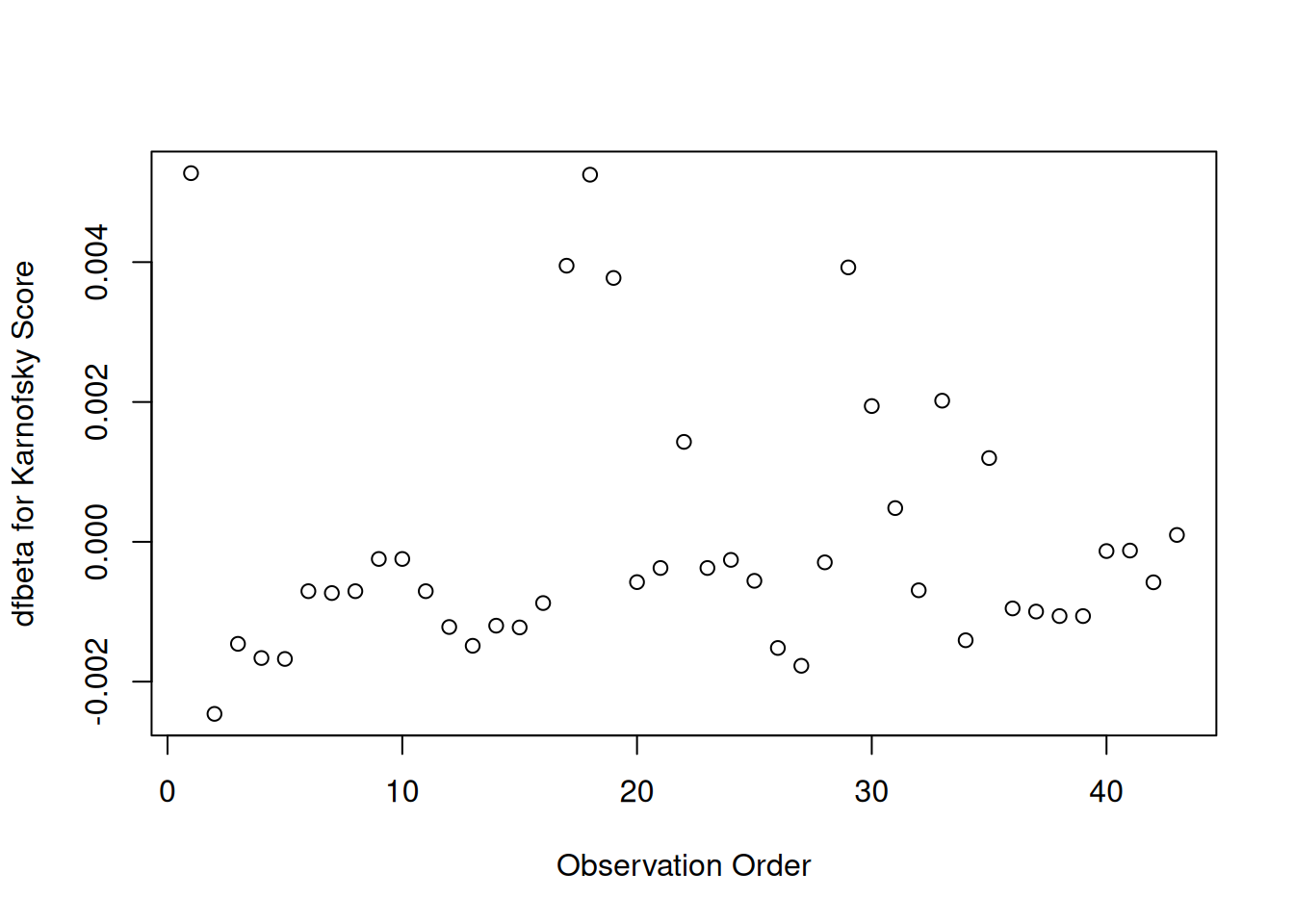
Karnofsky score

plot(hodg.dfb[,3],
     xlab="Observation Order",
     ylab="dfbeta for Karnofsky Score")

dfbeta Values by Observation Order for Karnofsky Score

The two highest dfbeta values for score are observations 1 and 18. The next three are observations 17, 29, and 19. The smallest value is observation 2.

Waiting time (dichotomized)

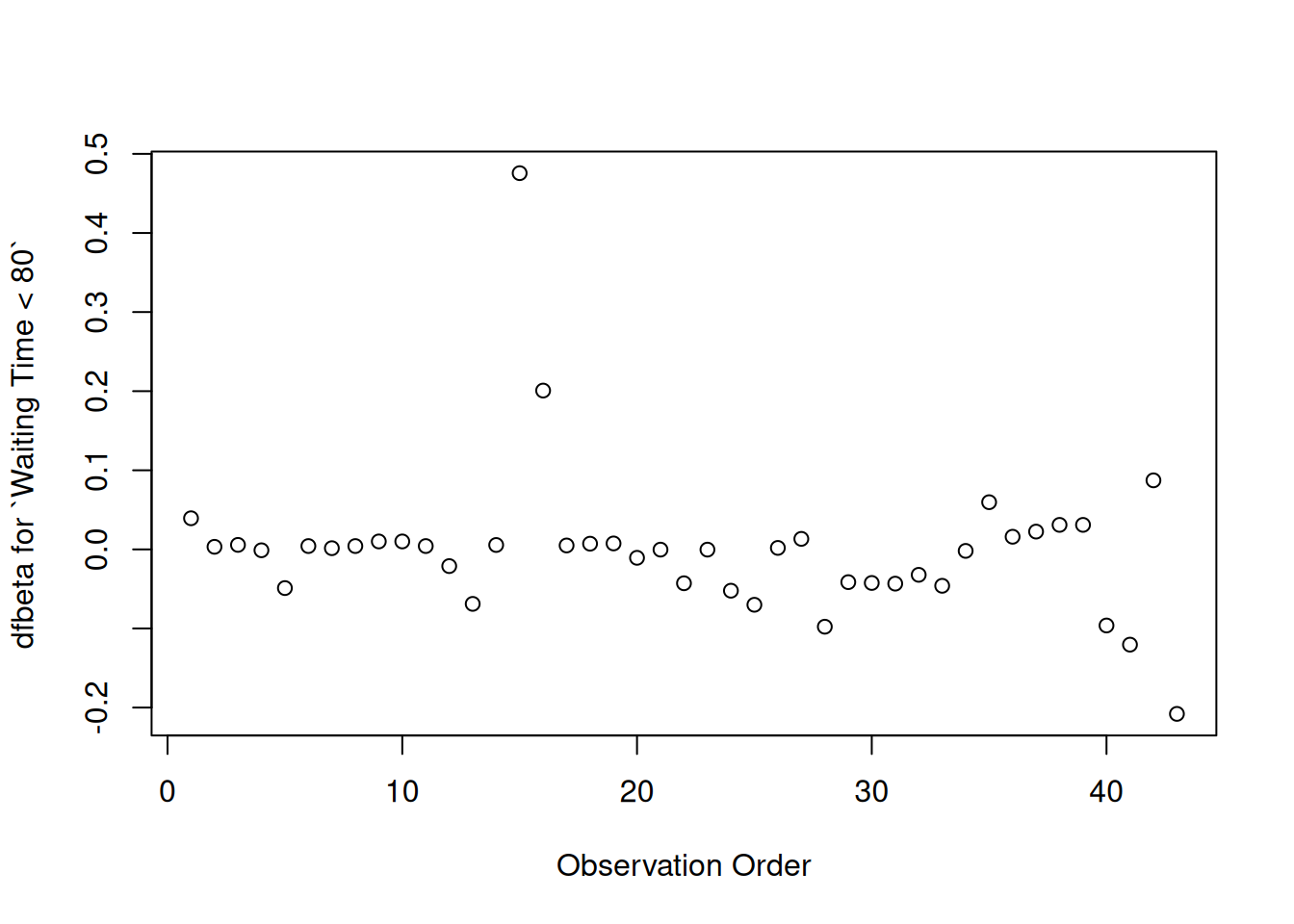
plot(
  hodg.dfb[,4],
  xlab="Observation Order",
  ylab="dfbeta for `Waiting Time < 80`")

dfbeta Values by Observation Order for Waiting Time (dichotomized)

The two large values of dfbeta for dichotomized waiting time are observations 15 and 16. This may have to do with the discretization of waiting time.

Interaction: graft type and disease type

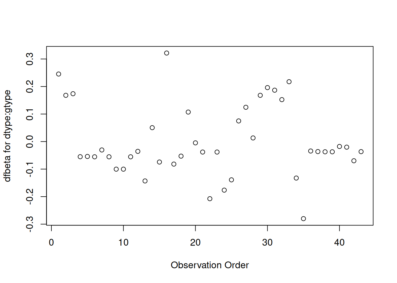
plot(hodg.dfb[,5],
     xlab="Observation Order",
     ylab="dfbeta for dtype:gtype")

dfbeta Values by Observation Order for dtype:gtype

The two largest values are observations 1 and 16. The smallest value is observation 35.

Table 2: Observations to Examine by Residuals and Influence

Diagnostic	Observations to Examine
Martingale Residuals	1, 29, 18
Deviance Residuals	1, 29
Graft Type Influence	1
Disease Type Influence	1, 16
Karnofsky Score Influence	1, 18 (17, 29, 19)
Waiting Time Influence	15, 16
Graft by Disease Influence	1, 16, 35

The most important observations to examine seem to be 1, 15, 16, 18, and 29.

with(hodg,summary(time[delta==1]))
#>    Min. 1st Qu.  Median    Mean 3rd Qu.    Max. 
#>     2.0    41.2    62.5    97.6    83.2   524.0

with(hodg,summary(wtime))
#>    Min. 1st Qu.  Median    Mean 3rd Qu.    Max. 
#>     5.0    16.0    24.0    37.7    55.5   171.0

with(hodg,summary(score))
#>    Min. 1st Qu.  Median    Mean 3rd Qu.    Max. 
#>    20.0    60.0    80.0    76.3    90.0   100.0

hodg.cox2
#> Call:
#> coxph(formula = Surv(time, event = delta == "dead") ~ gtype * 
#>     dtype + score + wt2, data = hodg2)
#> 
#>                                  coef exp(coef) se(coef)     z       p
#> gtypeAutologous                0.6651    1.9447   0.5943  1.12  0.2631
#> dtypeHodgkins                  2.3273   10.2505   0.7332  3.17  0.0015
#> score                         -0.0550    0.9464   0.0123 -4.46 8.2e-06
#> wt2long                       -2.0598    0.1275   1.0507 -1.96  0.0499
#> gtypeAutologous:dtypeHodgkins -2.0668    0.1266   0.9258 -2.23  0.0256
#> 
#> Likelihood ratio test=35.5  on 5 df, p=1.21e-06
#> n= 43, number of events= 26

hodg2[c(1,15,16,18,29),] |> 
  select(gtype, dtype, time, delta, score, wtime) |> 
  mutate(
    comment = 
      c(
        "early death, good score, low risk",
        "high risk grp, long wait, poor score",
        "high risk grp, short wait, poor score",
        "early death, good score, med risk grp",
        "early death, good score, med risk grp"
      ))

Action Items

• Unusual points may need checking, particularly if the data are not completely cleaned. In this case, observations 15 and 16 may show some trouble with the dichotomization of waiting time, but it still may be useful.
• The two largest residuals seem to be due to unexpectedly early deaths, but unfortunately this can occur.
• If hazards don’t look proportional, then we may need to use strata, between which the base hazards are permitted to be different. For this problem, the natural strata are the two diseases, because they could need to be managed differently anyway.
• A main point that we want to be sure of is the relative risk difference by disease type and graft type.

hodg.cox2 |> 
  predict(
    reference = "zero",
    newdata = means |> 
      mutate(
        wt2 = "short", 
        score = 0), 
    type = "lp") |> 
  data.frame('linear predictor' = _) |> 
  pander()

Linear Risk Predictors for Lymphoma

	linear.predictor
Non-Hodgkins,Allogenic	0
Non-Hodgkins,Autologous	0.6651
Hodgkins,Allogenic	2.327
Hodgkins,Autologous	0.9256

For Non-Hodgkin’s, the allogenic graft is better. For Hodgkin’s, the autologous graft is much better.

6.7 Stratified survival models

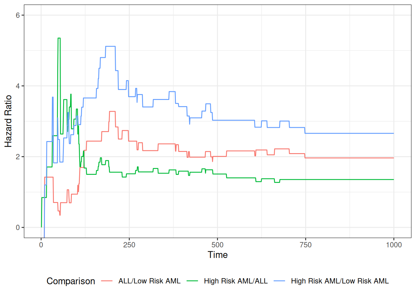
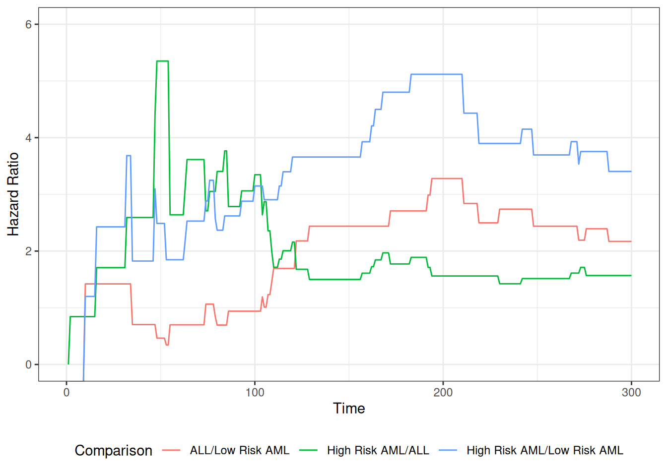
Revisiting the leukemia dataset (anderson)

We will analyze remission survival times on 42 leukemia patients, half on new treatment, half on standard treatment.

This is the same data as the drug6mp data from KMsurv, but with two other variables and without the pairing. This version comes from Kleinbaum and Klein (2012) (e.g., p281):

anderson = 
  paste0(
    "http://web1.sph.emory.edu/dkleinb/allDatasets/",
    "surv2datasets/anderson.dta") |> 
  haven::read_dta() |> 
  dplyr::mutate(
    status = status |> 
      case_match(
        1 ~ "relapse",
        0 ~ "censored"
      ),
    
    sex = sex |> 
      case_match(
        0 ~ "female",
        1 ~ "male"
      ) |> 
      factor() |> 
      relevel(ref = "female"),
    
    rx = rx |> 
      case_match(
        0 ~ "new",
        1 ~ "standard"
      ) |> 
      factor() |> relevel(ref = "standard"),
    
    surv = Surv(
      time = survt, 
      event = (status == "relapse"))
  )

print(anderson)

Cox semi-parametric proportional hazards model

anderson.cox1 = coxph(
  formula = surv ~ rx + sex + logwbc,
  data = anderson)

summary(anderson.cox1)
#> Call:
#> coxph(formula = surv ~ rx + sex + logwbc, data = anderson)
#> 
#>   n= 42, number of events= 30 
#> 
#>           coef exp(coef) se(coef)     z Pr(>|z|)    
#> rxnew   -1.504     0.222    0.462 -3.26   0.0011 ** 
#> sexmale  0.315     1.370    0.455  0.69   0.4887    
#> logwbc   1.682     5.376    0.337  5.00  5.8e-07 ***
#> ---
#> Signif. codes:  0 '***' 0.001 '**' 0.01 '*' 0.05 '.' 0.1 ' ' 1
#> 
#>         exp(coef) exp(-coef) lower .95 upper .95
#> rxnew       0.222      4.498     0.090     0.549
#> sexmale     1.370      0.730     0.562     3.338
#> logwbc      5.376      0.186     2.779    10.398
#> 
#> Concordance= 0.851  (se = 0.041 )
#> Likelihood ratio test= 47.2  on 3 df,   p=3e-10
#> Wald test            = 33.5  on 3 df,   p=2e-07
#> Score (logrank) test = 48  on 3 df,   p=2e-10

Test the proportional hazards assumption

cox.zph(anderson.cox1)
#>        chisq df    p
#> rx     0.036  1 0.85
#> sex    5.420  1 0.02
#> logwbc 0.142  1 0.71
#> GLOBAL 5.879  3 0.12

Graph the K-M survival curves

anderson_km_model = survfit(
  formula = surv ~ sex,
  data = anderson)

anderson_km_model |> 
  autoplot(conf.int = FALSE) +
  theme_bw() +
  theme(legend.position="bottom")

The survival curves cross, which indicates a problem in the proportionality assumption by sex.

Graph the Nelson-Aalen cumulative hazard

We can also look at the log-hazard (“cloglog survival”) plots:

anderson_na_model = survfit(
  formula = surv ~ sex,
  data = anderson,
  type = "fleming")

anderson_na_model |> 
  autoplot(
    fun = "cumhaz",
    conf.int = FALSE) +
  theme_classic() +
  theme(legend.position="bottom") +
  ylab("log(Cumulative Hazard)") +
  scale_y_continuous(
    trans = "log10",
    name = "Cumulative hazard (H(t), log scale)") +
  scale_x_continuous(
    breaks = c(1,2,5,10,20,50),
    trans = "log"
  )

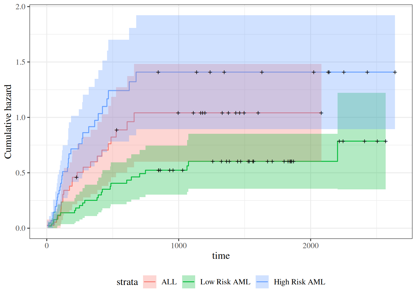
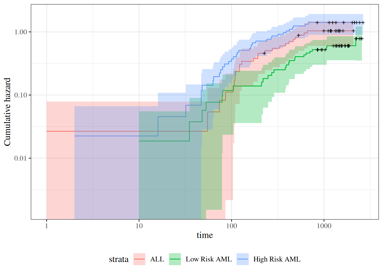
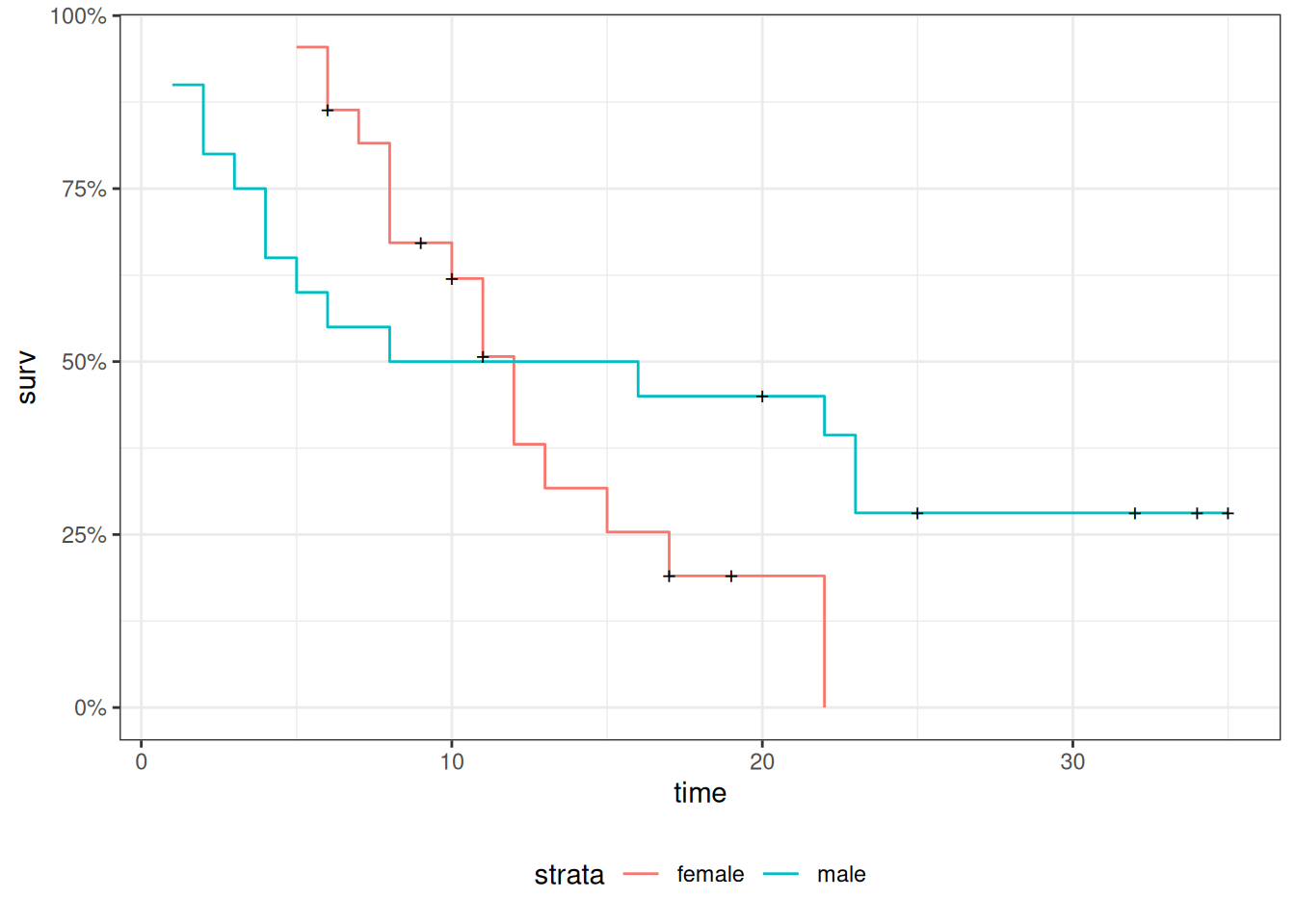
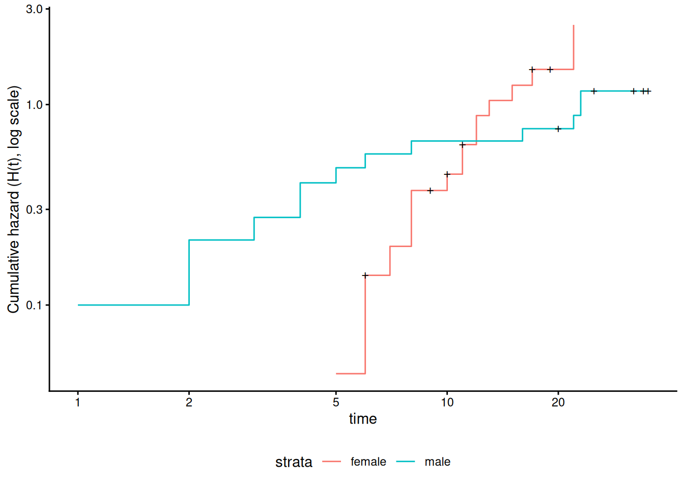
Figure 12: Cumulative hazard (cloglog scale) for anderson data

This can be fixed by using strata or possibly by other model alterations.

The Stratified Cox Model

• In a stratified Cox model, each stratum, defined by one or more factors, has its own base survival function \({\lambda}_0(t)\).
• But the coefficients for each variable not used in the strata definitions are assumed to be the same across strata.
• To check if this assumption is reasonable one can include interactions with strata and see if they are significant (this may generate a warning and NA lines but these can be ignored).
• Since the sex variable shows possible non-proportionality, we try stratifying on sex.

anderson.coxph.strat = 
  coxph(
    formula = 
      surv ~ rx + logwbc + strata(sex),
    data = anderson)

summary(anderson.coxph.strat)
#> Call:
#> coxph(formula = surv ~ rx + logwbc + strata(sex), data = anderson)
#> 
#>   n= 42, number of events= 30 
#> 
#>          coef exp(coef) se(coef)     z Pr(>|z|)    
#> rxnew  -0.998     0.369    0.474 -2.11    0.035 *  
#> logwbc  1.454     4.279    0.344  4.22  2.4e-05 ***
#> ---
#> Signif. codes:  0 '***' 0.001 '**' 0.01 '*' 0.05 '.' 0.1 ' ' 1
#> 
#>        exp(coef) exp(-coef) lower .95 upper .95
#> rxnew      0.369      2.713     0.146     0.932
#> logwbc     4.279      0.234     2.180     8.398
#> 
#> Concordance= 0.812  (se = 0.059 )
#> Likelihood ratio test= 32.1  on 2 df,   p=1e-07
#> Wald test            = 22.8  on 2 df,   p=1e-05
#> Score (logrank) test = 30.8  on 2 df,   p=2e-07

Let’s compare this to a model fit only on the subset of males:

anderson.coxph.male = 
  coxph(
    formula = surv ~ rx + logwbc,
    subset = sex == "male",
    data = anderson)

summary(anderson.coxph.male)
#> Call:
#> coxph(formula = surv ~ rx + logwbc, data = anderson, subset = sex == 
#>     "male")
#> 
#>   n= 20, number of events= 14 
#> 
#>          coef exp(coef) se(coef)     z Pr(>|z|)   
#> rxnew  -1.978     0.138    0.739 -2.68   0.0075 **
#> logwbc  1.743     5.713    0.536  3.25   0.0011 **
#> ---
#> Signif. codes:  0 '***' 0.001 '**' 0.01 '*' 0.05 '.' 0.1 ' ' 1
#> 
#>        exp(coef) exp(-coef) lower .95 upper .95
#> rxnew      0.138      7.227    0.0325     0.589
#> logwbc     5.713      0.175    1.9991    16.328
#> 
#> Concordance= 0.905  (se = 0.043 )
#> Likelihood ratio test= 29.2  on 2 df,   p=5e-07
#> Wald test            = 15.3  on 2 df,   p=5e-04
#> Score (logrank) test = 26.4  on 2 df,   p=2e-06

anderson.coxph.female = 
  coxph(
    formula = 
      surv ~ rx + logwbc,
    subset = sex == "female",
    data = anderson)

summary(anderson.coxph.female)
#> Call:
#> coxph(formula = surv ~ rx + logwbc, data = anderson, subset = sex == 
#>     "female")
#> 
#>   n= 22, number of events= 16 
#> 
#>          coef exp(coef) se(coef)     z Pr(>|z|)  
#> rxnew  -0.311     0.733    0.564 -0.55    0.581  
#> logwbc  1.206     3.341    0.503  2.40    0.017 *
#> ---
#> Signif. codes:  0 '***' 0.001 '**' 0.01 '*' 0.05 '.' 0.1 ' ' 1
#> 
#>        exp(coef) exp(-coef) lower .95 upper .95
#> rxnew      0.733      1.365     0.243      2.21
#> logwbc     3.341      0.299     1.245      8.96
#> 
#> Concordance= 0.692  (se = 0.085 )
#> Likelihood ratio test= 6.65  on 2 df,   p=0.04
#> Wald test            = 6.36  on 2 df,   p=0.04
#> Score (logrank) test = 6.74  on 2 df,   p=0.03

The coefficients of treatment look different. Are they statistically different?

anderson.coxph.strat.intxn = 
  coxph(
    formula = surv ~ strata(sex) * (rx + logwbc),
    data = anderson)

anderson.coxph.strat.intxn |> summary()
#> Call:
#> coxph(formula = surv ~ strata(sex) * (rx + logwbc), data = anderson)
#> 
#>   n= 42, number of events= 30 
#> 
#>                          coef exp(coef) se(coef)     z Pr(>|z|)  
#> rxnew                  -0.311     0.733    0.564 -0.55    0.581  
#> logwbc                  1.206     3.341    0.503  2.40    0.017 *
#> strata(sex)male:rxnew  -1.667     0.189    0.930 -1.79    0.073 .
#> strata(sex)male:logwbc  0.537     1.710    0.735  0.73    0.465  
#> ---
#> Signif. codes:  0 '***' 0.001 '**' 0.01 '*' 0.05 '.' 0.1 ' ' 1
#> 
#>                        exp(coef) exp(-coef) lower .95 upper .95
#> rxnew                      0.733      1.365    0.2427      2.21
#> logwbc                     3.341      0.299    1.2452      8.96
#> strata(sex)male:rxnew      0.189      5.294    0.0305      1.17
#> strata(sex)male:logwbc     1.710      0.585    0.4048      7.23
#> 
#> Concordance= 0.797  (se = 0.058 )
#> Likelihood ratio test= 35.8  on 4 df,   p=3e-07
#> Wald test            = 21.7  on 4 df,   p=2e-04
#> Score (logrank) test = 33.1  on 4 df,   p=1e-06

anova(
  anderson.coxph.strat.intxn,
  anderson.coxph.strat)

We don’t have enough evidence to tell the difference between these two models.

Conclusions

• We chose to use a stratified model because of the apparent non-proportionality of the hazard for the sex variable.
• When we fit interactions with the strata variable, we did not get an improved model (via the likelihood ratio test).
• So we use the stratifed model with coefficients that are the same across strata.

Another Modeling Approach

• We used an additive model without interactions and saw that we might need to stratify by sex.
• Instead, we could try to improve the model’s functional form - maybe the interaction of treatment and sex is real, and after fitting that we might not need separate hazard functions.
• Either approach may work.

anderson.coxph.intxn = 
  coxph(
    formula = surv ~ (rx + logwbc) * sex,
    data = anderson)

anderson.coxph.intxn |> summary()
#> Call:
#> coxph(formula = surv ~ (rx + logwbc) * sex, data = anderson)
#> 
#>   n= 42, number of events= 30 
#> 
#>                   coef exp(coef) se(coef)     z Pr(>|z|)  
#> rxnew          -0.3748    0.6874   0.5545 -0.68    0.499  
#> logwbc          1.0637    2.8971   0.4726  2.25    0.024 *
#> sexmale        -2.8052    0.0605   2.0323 -1.38    0.167  
#> rxnew:sexmale  -2.1782    0.1132   0.9109 -2.39    0.017 *
#> logwbc:sexmale  1.2303    3.4223   0.6301  1.95    0.051 .
#> ---
#> Signif. codes:  0 '***' 0.001 '**' 0.01 '*' 0.05 '.' 0.1 ' ' 1
#> 
#>                exp(coef) exp(-coef) lower .95 upper .95
#> rxnew             0.6874      1.455   0.23185     2.038
#> logwbc            2.8971      0.345   1.14730     7.315
#> sexmale           0.0605     16.531   0.00113     3.248
#> rxnew:sexmale     0.1132      8.830   0.01899     0.675
#> logwbc:sexmale    3.4223      0.292   0.99539    11.766
#> 
#> Concordance= 0.861  (se = 0.036 )
#> Likelihood ratio test= 57  on 5 df,   p=5e-11
#> Wald test            = 35.6  on 5 df,   p=1e-06
#> Score (logrank) test = 57.1  on 5 df,   p=5e-11

cox.zph(anderson.coxph.intxn)
#>            chisq df    p
#> rx         0.136  1 0.71
#> logwbc     1.652  1 0.20
#> sex        1.266  1 0.26
#> rx:sex     0.149  1 0.70
#> logwbc:sex 0.102  1 0.75
#> GLOBAL     3.747  5 0.59

6.8 Time-varying covariates

(adapted from Klein and Moeschberger (2003), §9.2)

Motivating example: back to the leukemia dataset

# load the data:
data(bmt, package = 'KMsurv')
bmt |> as_tibble() |> print(n = 5)
#> # A tibble: 137 × 22
#>   group    t1    t2    d1    d2    d3    ta    da    tc    dc    tp    dp    z1
#>   <int> <int> <int> <int> <int> <int> <int> <int> <int> <int> <int> <int> <int>
#> 1     1  2081  2081     0     0     0    67     1   121     1    13     1    26
#> 2     1  1602  1602     0     0     0  1602     0   139     1    18     1    21
#> 3     1  1496  1496     0     0     0  1496     0   307     1    12     1    26
#> 4     1  1462  1462     0     0     0    70     1    95     1    13     1    17
#> 5     1  1433  1433     0     0     0  1433     0   236     1    12     1    32
#> # ℹ 132 more rows
#> # ℹ 9 more variables: z2 <int>, z3 <int>, z4 <int>, z5 <int>, z6 <int>,
#> #   z7 <int>, z8 <int>, z9 <int>, z10 <int>

This dataset comes from the Copelan et al. (1991) study of allogenic bone marrow transplant therapy for acute myeloid leukemia (AML) and acute lymphoblastic leukemia (ALL).

Outcomes (endpoints)

• The main endpoint is disease-free survival (t2 and d3) for the three risk groups, “ALL”, “AML Low Risk”, and “AML High Risk”.

Possible intermediate events

• graft vs. host disease (GVHD), an immunological rejection response to the transplant (bad)
• acute (AGVHD)
• chronic (CGVHD)
• platelet recovery, a return of platelet count to normal levels (good)

One or the other, both in either order, or neither may occur.

Covariates

• We are interested in possibly using the covariates z1-z10 to adjust for other factors.

• In addition, the time-varying covariates for acute GVHD, chronic GVHD, and platelet recovery may be useful.

Preprocessing

We reformat the data before analysis:

# reformat the data:
bmt1 = 
  bmt |> 
  as_tibble() |> 
  mutate(
    id = 1:n(), # will be used to connect multiple records for the same individual
    
    group =  group |> 
      case_match(
        1 ~ "ALL",
        2 ~ "Low Risk AML",
        3 ~ "High Risk AML") |> 
      factor(levels = c("ALL", "Low Risk AML", "High Risk AML")),
    
    `patient age` = z1,
    
    `donor age` = z2,
    
    `patient sex` = z3 |> 
      case_match(
        0 ~ "Female",
        1 ~ "Male"),
    
    `donor sex` = z4 |> 
      case_match(
        0 ~ "Female",
        1 ~ "Male"),
    
    `Patient CMV Status` = z5 |> 
      case_match(
        0 ~ "CMV Negative",
        1 ~ "CMV Positive"),
    
    `Donor CMV Status` = z6 |> 
      case_match(
        0 ~ "CMV Negative",
        1 ~ "CMV Positive"),
    
    `Waiting Time to Transplant` = z7,
    
    FAB = z8 |> 
      case_match(
        1 ~ "Grade 4 Or 5 (AML only)",
        0 ~ "Other") |> 
      factor() |> 
      relevel(ref = "Other"),
    
    hospital = z9 |>  # `z9` is hospital
      case_match(
        1 ~ "Ohio State University",
        2 ~ "Alferd",
        3 ~ "St. Vincent",
        4 ~ "Hahnemann") |> 
      factor() |> 
      relevel(ref = "Ohio State University"),
    
    MTX = (z10 == 1) # a prophylatic treatment for GVHD
    
  ) |> 
  select(-(z1:z10)) # don't need these anymore

bmt1 |> 
  select(group, id:MTX) |> 
  print(n = 10)
#> # A tibble: 137 × 12
#>    group    id `patient age` `donor age` `patient sex` `donor sex`
#>    <fct> <int>         <int>       <int> <chr>         <chr>      
#>  1 ALL       1            26          33 Male          Female     
#>  2 ALL       2            21          37 Male          Male       
#>  3 ALL       3            26          35 Male          Male       
#>  4 ALL       4            17          21 Female        Male       
#>  5 ALL       5            32          36 Male          Male       
#>  6 ALL       6            22          31 Male          Male       
#>  7 ALL       7            20          17 Male          Female     
#>  8 ALL       8            22          24 Male          Female     
#>  9 ALL       9            18          21 Female        Male       
#> 10 ALL      10            24          40 Male          Male       
#> # ℹ 127 more rows
#> # ℹ 6 more variables: `Patient CMV Status` <chr>, `Donor CMV Status` <chr>,
#> #   `Waiting Time to Transplant` <int>, FAB <fct>, hospital <fct>, MTX <lgl>

Time-Dependent Covariates

• A time-dependent covariate (“TDC”) is a covariate whose value changes during the course of the study.
• For variables like age that change in a linear manner with time, we can just use the value at the start.
• But it may be plausible that when and if GVHD occurs, the risk of relapse or death increases, and when and if platelet recovery occurs, the risk decreases.

Analysis in R

• We form a variable precovery which is = 0 before platelet recovery and is = 1 after platelet recovery, if it occurs.
• For each subject where platelet recovery occurs, we set up multiple records (lines in the data frame); for example one from t = 0 to the time of platelet recovery, and one from that time to relapse, recovery, or death.
• We do the same for acute GVHD and chronic GVHD.
• For each record, the covariates are constant.

bmt2 = bmt1 |> 
  #set up new long-format data set:
  tmerge(bmt1, id = id, tstop = t2) |> 
  
  # the following three steps can be in any order, 
  # and will still produce the same result:
  #add aghvd as tdc:
  tmerge(bmt1, id = id, agvhd = tdc(ta)) |> 
  #add cghvd as tdc:
  tmerge(bmt1, id = id, cgvhd = tdc(tc)) |> 
  #add platelet recovery as tdc:
  tmerge(bmt1, id = id, precovery = tdc(tp))   

bmt2 = bmt2 |> 
  as_tibble() |> 
  mutate(status = as.numeric((tstop == t2) & d3))
# status only = 1 if at end of t2 and not censored

Let’s see how we’ve rearranged the first row of the data:

bmt1 |> 
  dplyr::filter(id == 1) |> 
  dplyr::select(id, t1, d1, t2, d2, d3, ta, da, tc, dc, tp, dp)

The event times for this individual are:

• t = 0 time of transplant
• tp = 13 platelet recovery
• ta = 67 acute GVHD onset
• tc = 121 chronic GVHD onset
• t2 = 2081 end of study, patient not relapsed or dead

After converting the data to long-format, we have:

bmt2 |> 
  select(
    id,
    tstart,
    tstop,
    agvhd,
    cgvhd,
    precovery,
    status
  ) |> 
  dplyr::filter(id == 1)

Note that status could have been 1 on the last row, indicating that relapse or death occurred; since it is false, the participant must have exited the study without experiencing relapse or death (i.e., they were censored).

Event sequences

Let:

• A = acute GVHD
• C = chronic GVHD
• P = platelet recovery

Each of the eight possible combinations of A or not-A, with C or not-C, with P or not-P occurs in this data set.

• A always occurs before C, and P always occurs before C, if both occur.
• Thus there are ten event sequences in the data set: None, A, C, P, AC, AP, PA, PC, APC, and PAC.
• In general, there could be as many as \(1+3+(3)(2)+6=16\) sequences, but our domain knowledge tells us that some are missing: CA, CP, CAP, CPA, PCA, PC, PAC
• Different subjects could have 1, 2, 3, or 4 intervals, depending on which of acute GVHD, chronic GVHD, and/or platelet recovery occurred.
• The final interval for any subject has status = 1 if the subject relapsed or died at that time; otherwise status = 0.
• Any earlier intervals have status = 0.
• Even though there might be multiple lines per ID in the dataset, there is never more than one event, so no alterations need be made in the estimation procedures or in the interpretation of the output.
• The function tmerge in the survival package eases the process of constructing the new long-format dataset.

Model with Time-Fixed Covariates

bmt1 = 
  bmt1 |> 
  mutate(surv = Surv(t2,d3))

bmt_coxph_TF = coxph(
  formula = surv ~ group + `patient age`*`donor age` + FAB,
  data = bmt1)
summary(bmt_coxph_TF)
#> Call:
#> coxph(formula = surv ~ group + `patient age` * `donor age` + 
#>     FAB, data = bmt1)
#> 
#>   n= 137, number of events= 83 
#> 
#>                                 coef exp(coef)  se(coef)     z Pr(>|z|)    
#> groupLow Risk AML          -1.090648  0.335999  0.354279 -3.08  0.00208 ** 
#> groupHigh Risk AML         -0.403905  0.667707  0.362777 -1.11  0.26555    
#> `patient age`              -0.081639  0.921605  0.036107 -2.26  0.02376 *  
#> `donor age`                -0.084587  0.918892  0.030097 -2.81  0.00495 ** 
#> FABGrade 4 Or 5 (AML only)  0.837416  2.310388  0.278464  3.01  0.00264 ** 
#> `patient age`:`donor age`   0.003159  1.003164  0.000951  3.32  0.00089 ***
#> ---
#> Signif. codes:  0 '***' 0.001 '**' 0.01 '*' 0.05 '.' 0.1 ' ' 1
#> 
#>                            exp(coef) exp(-coef) lower .95 upper .95
#> groupLow Risk AML              0.336      2.976     0.168     0.673
#> groupHigh Risk AML             0.668      1.498     0.328     1.360
#> `patient age`                  0.922      1.085     0.859     0.989
#> `donor age`                    0.919      1.088     0.866     0.975
#> FABGrade 4 Or 5 (AML only)     2.310      0.433     1.339     3.988
#> `patient age`:`donor age`      1.003      0.997     1.001     1.005
#> 
#> Concordance= 0.665  (se = 0.033 )
#> Likelihood ratio test= 32.8  on 6 df,   p=1e-05
#> Wald test            = 33  on 6 df,   p=1e-05
#> Score (logrank) test = 35.8  on 6 df,   p=3e-06
drop1(bmt_coxph_TF, test = "Chisq")

bmt1$mres = 
  bmt_coxph_TF |> 
  update(. ~ . - `donor age`) |> 
  residuals(type="martingale")

bmt1 |> 
  ggplot(aes(x = `donor age`, y = mres)) +
  geom_point() +
  geom_smooth(method = "loess", aes(col = "loess")) +
  geom_smooth(method = 'lm', aes(col = "lm")) +
  theme_classic() +
  xlab("Donor age") +
  ylab("Martingale Residuals") +
  guides(col=guide_legend(title = ""))

Martingale residuals for Donor age

A more complex functional form for donor age seems warranted; left as an exercise for the reader.

Now we will add the time-varying covariates:

# add counting process formulation of Surv():
bmt2 = 
  bmt2 |> 
  mutate(
    surv = 
      Surv(
        time = tstart,
        time2 = tstop,
        event = status,
        type = "counting"))

Let’s see how the data looks for patient 15:

bmt1 |> dplyr::filter(id == 15) |> dplyr::select(tp, dp, tc,dc, ta, da, FAB, surv, t1, d1, t2, d2, d3)

bmt2 |> dplyr::filter(id == 15) |> dplyr::select(id, agvhd, cgvhd, precovery, surv)

Model with Time-Dependent Covariates

bmt_coxph_TV = coxph(
  formula = 
    surv ~ 
    group + `patient age`*`donor age` + FAB + agvhd + cgvhd + precovery,
  data = bmt2)

summary(bmt_coxph_TV)
#> Call:
#> coxph(formula = surv ~ group + `patient age` * `donor age` + 
#>     FAB + agvhd + cgvhd + precovery, data = bmt2)
#> 
#>   n= 341, number of events= 83 
#> 
#>                                 coef exp(coef)  se(coef)     z Pr(>|z|)   
#> groupLow Risk AML          -1.038514  0.353980  0.358220 -2.90   0.0037 **
#> groupHigh Risk AML         -0.380481  0.683533  0.374867 -1.01   0.3101   
#> `patient age`              -0.073351  0.929275  0.035956 -2.04   0.0413 * 
#> `donor age`                -0.076406  0.926440  0.030196 -2.53   0.0114 * 
#> FABGrade 4 Or 5 (AML only)  0.805700  2.238263  0.284273  2.83   0.0046 **
#> agvhd                       0.150565  1.162491  0.306848  0.49   0.6237   
#> cgvhd                      -0.116136  0.890354  0.289046 -0.40   0.6878   
#> precovery                  -0.941123  0.390190  0.347861 -2.71   0.0068 **
#> `patient age`:`donor age`   0.002895  1.002899  0.000944  3.07   0.0022 **
#> ---
#> Signif. codes:  0 '***' 0.001 '**' 0.01 '*' 0.05 '.' 0.1 ' ' 1
#> 
#>                            exp(coef) exp(-coef) lower .95 upper .95
#> groupLow Risk AML              0.354      2.825     0.175     0.714
#> groupHigh Risk AML             0.684      1.463     0.328     1.425
#> `patient age`                  0.929      1.076     0.866     0.997
#> `donor age`                    0.926      1.079     0.873     0.983
#> FABGrade 4 Or 5 (AML only)     2.238      0.447     1.282     3.907
#> agvhd                          1.162      0.860     0.637     2.121
#> cgvhd                          0.890      1.123     0.505     1.569
#> precovery                      0.390      2.563     0.197     0.772
#> `patient age`:`donor age`      1.003      0.997     1.001     1.005
#> 
#> Concordance= 0.702  (se = 0.028 )
#> Likelihood ratio test= 40.3  on 9 df,   p=7e-06
#> Wald test            = 42.4  on 9 df,   p=3e-06
#> Score (logrank) test = 47.2  on 9 df,   p=4e-07

Platelet recovery is highly significant.

Neither acute GVHD (agvhd) nor chronic GVHD (cgvhd) has a statistically significant effect here, nor are they significant in models with the other one removed.

update(bmt_coxph_TV, .~.-agvhd) |> summary()
#> Call:
#> coxph(formula = surv ~ group + `patient age` + `donor age` + 
#>     FAB + cgvhd + precovery + `patient age`:`donor age`, data = bmt2)
#> 
#>   n= 341, number of events= 83 
#> 
#>                                 coef exp(coef)  se(coef)     z Pr(>|z|)   
#> groupLow Risk AML          -1.049870  0.349983  0.356727 -2.94   0.0032 **
#> groupHigh Risk AML         -0.417049  0.658988  0.365348 -1.14   0.2537   
#> `patient age`              -0.070749  0.931696  0.035477 -1.99   0.0461 * 
#> `donor age`                -0.075693  0.927101  0.030075 -2.52   0.0118 * 
#> FABGrade 4 Or 5 (AML only)  0.807035  2.241253  0.283437  2.85   0.0044 **
#> cgvhd                      -0.095393  0.909015  0.285979 -0.33   0.7387   
#> precovery                  -0.983653  0.373942  0.338170 -2.91   0.0036 **
#> `patient age`:`donor age`   0.002859  1.002863  0.000936  3.05   0.0023 **
#> ---
#> Signif. codes:  0 '***' 0.001 '**' 0.01 '*' 0.05 '.' 0.1 ' ' 1
#> 
#>                            exp(coef) exp(-coef) lower .95 upper .95
#> groupLow Risk AML              0.350      2.857     0.174     0.704
#> groupHigh Risk AML             0.659      1.517     0.322     1.349
#> `patient age`                  0.932      1.073     0.869     0.999
#> `donor age`                    0.927      1.079     0.874     0.983
#> FABGrade 4 Or 5 (AML only)     2.241      0.446     1.286     3.906
#> cgvhd                          0.909      1.100     0.519     1.592
#> precovery                      0.374      2.674     0.193     0.726
#> `patient age`:`donor age`      1.003      0.997     1.001     1.005
#> 
#> Concordance= 0.701  (se = 0.027 )
#> Likelihood ratio test= 40  on 8 df,   p=3e-06
#> Wald test            = 42.4  on 8 df,   p=1e-06
#> Score (logrank) test = 47.2  on 8 df,   p=1e-07
update(bmt_coxph_TV, .~.-cgvhd) |> summary()
#> Call:
#> coxph(formula = surv ~ group + `patient age` + `donor age` + 
#>     FAB + agvhd + precovery + `patient age`:`donor age`, data = bmt2)
#> 
#>   n= 341, number of events= 83 
#> 
#>                                 coef exp(coef)  se(coef)     z Pr(>|z|)   
#> groupLow Risk AML          -1.019638  0.360725  0.355311 -2.87   0.0041 **
#> groupHigh Risk AML         -0.381356  0.682935  0.374568 -1.02   0.3086   
#> `patient age`              -0.073189  0.929426  0.035890 -2.04   0.0414 * 
#> `donor age`                -0.076753  0.926118  0.030121 -2.55   0.0108 * 
#> FABGrade 4 Or 5 (AML only)  0.811716  2.251769  0.284012  2.86   0.0043 **
#> agvhd                       0.131621  1.140676  0.302623  0.43   0.6636   
#> precovery                  -0.946697  0.388021  0.347265 -2.73   0.0064 **
#> `patient age`:`donor age`   0.002904  1.002908  0.000943  3.08   0.0021 **
#> ---
#> Signif. codes:  0 '***' 0.001 '**' 0.01 '*' 0.05 '.' 0.1 ' ' 1
#> 
#>                            exp(coef) exp(-coef) lower .95 upper .95
#> groupLow Risk AML              0.361      2.772     0.180     0.724
#> groupHigh Risk AML             0.683      1.464     0.328     1.423
#> `patient age`                  0.929      1.076     0.866     0.997
#> `donor age`                    0.926      1.080     0.873     0.982
#> FABGrade 4 Or 5 (AML only)     2.252      0.444     1.291     3.929
#> agvhd                          1.141      0.877     0.630     2.064
#> precovery                      0.388      2.577     0.196     0.766
#> `patient age`:`donor age`      1.003      0.997     1.001     1.005
#> 
#> Concordance= 0.701  (se = 0.027 )
#> Likelihood ratio test= 40.1  on 8 df,   p=3e-06
#> Wald test            = 42.1  on 8 df,   p=1e-06
#> Score (logrank) test = 47.1  on 8 df,   p=1e-07

Let’s drop them both:

bmt_coxph_TV2 = update(bmt_coxph_TV, . ~ . - agvhd -cgvhd)
bmt_coxph_TV2 |> summary()
#> Call:
#> coxph(formula = surv ~ group + `patient age` + `donor age` + 
#>     FAB + precovery + `patient age`:`donor age`, data = bmt2)
#> 
#>   n= 341, number of events= 83 
#> 
#>                                 coef exp(coef)  se(coef)     z Pr(>|z|)   
#> groupLow Risk AML          -1.032520  0.356108  0.353202 -2.92   0.0035 **
#> groupHigh Risk AML         -0.413888  0.661075  0.365209 -1.13   0.2571   
#> `patient age`              -0.070965  0.931495  0.035453 -2.00   0.0453 * 
#> `donor age`                -0.076052  0.926768  0.030007 -2.53   0.0113 * 
#> FABGrade 4 Or 5 (AML only)  0.811926  2.252242  0.283231  2.87   0.0041 **
#> precovery                  -0.983505  0.373998  0.337997 -2.91   0.0036 **
#> `patient age`:`donor age`   0.002872  1.002876  0.000936  3.07   0.0021 **
#> ---
#> Signif. codes:  0 '***' 0.001 '**' 0.01 '*' 0.05 '.' 0.1 ' ' 1
#> 
#>                            exp(coef) exp(-coef) lower .95 upper .95
#> groupLow Risk AML              0.356      2.808     0.178     0.712
#> groupHigh Risk AML             0.661      1.513     0.323     1.352
#> `patient age`                  0.931      1.074     0.869     0.999
#> `donor age`                    0.927      1.079     0.874     0.983
#> FABGrade 4 Or 5 (AML only)     2.252      0.444     1.293     3.924
#> precovery                      0.374      2.674     0.193     0.725
#> `patient age`:`donor age`      1.003      0.997     1.001     1.005
#> 
#> Concordance= 0.7  (se = 0.027 )
#> Likelihood ratio test= 39.9  on 7 df,   p=1e-06
#> Wald test            = 42.2  on 7 df,   p=5e-07
#> Score (logrank) test = 47.1  on 7 df,   p=5e-08

6.9 Recurrent Events

(Adapted from Kleinbaum and Klein (2012), Ch 8)

• Sometimes an appropriate analysis requires consideration of recurrent events.
• A patient with arthritis may have more than one flareup. The same is true of many recurring-remitting diseases.
• In this case, we have more than one line in the data frame, but each line may have an event.
• We have to use a “robust” variance estimator to account for correlation of time-to-events within a patient.

Bladder Cancer Data Set

The bladder cancer dataset from Kleinbaum and Klein (2012) contains recurrent event outcome information for eighty-six cancer patients followed for the recurrence of bladder cancer tumor after transurethral surgical excision (Byar and Green 1980). The exposure of interest is the effect of the drug treatment of thiotepa. Control variables are the initial number and initial size of tumors. The data layout is suitable for a counting processes approach.

This drug is still a possible choice for some patients. Another therapeutic choice is Bacillus Calmette-Guerin (BCG), a live bacterium related to cow tuberculosis.

Data dictionary

Variables in the bladder dataset

Variable	Definition
id	Patient unique ID
status	for each time interval: 1 = recurred, 0 = censored
interval	1 = first recurrence, etc.
intime	`tstop - tstart (all times in months)
tstart	start of interval
tstop	end of interval
tx	treatment code, 1 = thiotepa
num	number of initial tumors
size	size of initial tumors (cm)

• There are 85 patients and 190 lines in the dataset, meaning that many patients have more than one line.
• Patient 1 with 0 observation time was removed.
• Of the 85 patients, 47 had at least one recurrence and 38 had none.
• 18 patients had exactly one recurrence.
• There were up to 4 recurrences in a patient.
• Of the 190 intervals, 112 terminated with a recurrence and 78 were censored.

Different intervals for the same patient are correlated.

• Is the effective sample size 47 or 112? This might narrow confidence intervals by as much as a factor of \(\sqrt{112/47}=1.54\)

• What happens if I have 5 treatment and 5 control values and want to do a t-test and I then duplicate the 10 values as if the sample size was 20? This falsely narrows confidence intervals by a factor of \(\sqrt{2}=1.41\).

bladder = 
  paste0(
    "http://web1.sph.emory.edu/dkleinb/allDatasets",
    "/surv2datasets/bladder.dta") |> 
  read_dta() |> 
  as_tibble()

bladder = bladder[-1,]  #remove subject with 0 observation time
print(bladder)

bladder = 
  bladder |> 
  mutate(
    surv = 
      Surv(
        time = start,
        time2 = stop,
        event = event,
        type = "counting"))

bladder.cox1 = coxph(
  formula = surv~tx+num+size,
  data = bladder)

#results with biased variance-covariance matrix:
summary(bladder.cox1)
#> Call:
#> coxph(formula = surv ~ tx + num + size, data = bladder)
#> 
#>   n= 190, number of events= 112 
#> 
#>         coef exp(coef) se(coef)     z Pr(>|z|)    
#> tx   -0.4116    0.6626   0.1999 -2.06  0.03947 *  
#> num   0.1637    1.1778   0.0478  3.43  0.00061 ***
#> size -0.0411    0.9598   0.0703 -0.58  0.55897    
#> ---
#> Signif. codes:  0 '***' 0.001 '**' 0.01 '*' 0.05 '.' 0.1 ' ' 1
#> 
#>      exp(coef) exp(-coef) lower .95 upper .95
#> tx       0.663      1.509     0.448      0.98
#> num      1.178      0.849     1.073      1.29
#> size     0.960      1.042     0.836      1.10
#> 
#> Concordance= 0.624  (se = 0.032 )
#> Likelihood ratio test= 14.7  on 3 df,   p=0.002
#> Wald test            = 15.9  on 3 df,   p=0.001
#> Score (logrank) test = 16.2  on 3 df,   p=0.001

Note

The likelihood ratio and score tests assume independence of observations within a cluster. The Wald and robust score tests do not.

adding cluster = id

If we add cluster= id to the call to coxph, the coefficient estimates don’t change, but we get an additional column in the summary() output: robust se:

bladder.cox2 = coxph(
  formula = surv ~ tx + num + size,
  cluster = id,
  data = bladder)

#unbiased though this reduces power:
summary(bladder.cox2)
#> Call:
#> coxph(formula = surv ~ tx + num + size, data = bladder, cluster = id)
#> 
#>   n= 190, number of events= 112 
#> 
#>         coef exp(coef) se(coef) robust se     z Pr(>|z|)   
#> tx   -0.4116    0.6626   0.1999    0.2488 -1.65   0.0980 . 
#> num   0.1637    1.1778   0.0478    0.0584  2.80   0.0051 **
#> size -0.0411    0.9598   0.0703    0.0742 -0.55   0.5799   
#> ---
#> Signif. codes:  0 '***' 0.001 '**' 0.01 '*' 0.05 '.' 0.1 ' ' 1
#> 
#>      exp(coef) exp(-coef) lower .95 upper .95
#> tx       0.663      1.509     0.407      1.08
#> num      1.178      0.849     1.050      1.32
#> size     0.960      1.042     0.830      1.11
#> 
#> Concordance= 0.624  (se = 0.031 )
#> Likelihood ratio test= 14.7  on 3 df,   p=0.002
#> Wald test            = 11.2  on 3 df,   p=0.01
#> Score (logrank) test = 16.2  on 3 df,   p=0.001,   Robust = 10.8  p=0.01
#> 
#>   (Note: the likelihood ratio and score tests assume independence of
#>      observations within a cluster, the Wald and robust score tests do not).

robust se is larger than se, and accounts for the repeated observations from the same individuals:

round(bladder.cox2$naive.var, 4)
#>         [,1]    [,2]   [,3]
#> [1,]  0.0400 -0.0014 0.0000
#> [2,] -0.0014  0.0023 0.0007
#> [3,]  0.0000  0.0007 0.0049
round(bladder.cox2$var, 4)
#>         [,1]    [,2]    [,3]
#> [1,]  0.0619 -0.0026 -0.0004
#> [2,] -0.0026  0.0034  0.0013
#> [3,] -0.0004  0.0013  0.0055

These are the ratios of correct confidence intervals to naive ones:

with(bladder.cox2, diag(var)/diag(naive.var)) |> sqrt()
#> [1] 1.24449 1.22309 1.05576

We might try dropping the non-significant size variable:

#remove non-significant size variable:
bladder.cox3 = bladder.cox2 |> update(. ~ . - size)
summary(bladder.cox3)
#> Call:
#> coxph(formula = surv ~ tx + num, data = bladder, cluster = id)
#> 
#>   n= 190, number of events= 112 
#> 
#>        coef exp(coef) se(coef) robust se     z Pr(>|z|)   
#> tx  -0.4117    0.6625   0.2003    0.2515 -1.64   0.1017   
#> num  0.1700    1.1853   0.0465    0.0564  3.02   0.0026 **
#> ---
#> Signif. codes:  0 '***' 0.001 '**' 0.01 '*' 0.05 '.' 0.1 ' ' 1
#> 
#>     exp(coef) exp(-coef) lower .95 upper .95
#> tx      0.663      1.509     0.405      1.08
#> num     1.185      0.844     1.061      1.32
#> 
#> Concordance= 0.623  (se = 0.031 )
#> Likelihood ratio test= 14.3  on 2 df,   p=8e-04
#> Wald test            = 10.2  on 2 df,   p=0.006
#> Score (logrank) test = 15.8  on 2 df,   p=4e-04,   Robust = 10.6  p=0.005
#> 
#>   (Note: the likelihood ratio and score tests assume independence of
#>      observations within a cluster, the Wald and robust score tests do not).

Ways to check PH assumption:

• cloglog
• schoenfeld residuals
• interaction with time

6.10 Age as the time scale

See Canchola et al. (2003).

Canchola, Alison J, Susan L Stewart, Leslie Bernstein, et al. 2003. “Cox Regression Using Different Time-Scales.” Western Users of SAS Software (San Francisco, California). https://www.lexjansen.com/wuss/2003/DataAnalysis/i-cox_time_scales.pdf.

Copelan, Edward A, James C Biggs, James M Thompson, et al. 1991. Treatment for Acute Myelocytic Leukemia with Allogeneic Bone Marrow Transplantation Following Preparation with BuCy2. https://doi.org/10.1182/blood.V78.3.838.838.

Dobson, Annette J, and Adrian G Barnett. 2018. An Introduction to Generalized Linear Models. 4th ed. CRC press. https://doi.org/10.1201/9781315182780.

Grambsch, Patricia M, and Terry M Therneau. 1994. “Proportional Hazards Tests and Diagnostics Based on Weighted Residuals.” Biometrika 81 (3): 515–26. https://doi.org/10.1093/biomet/81.3.515.

Klein, John P, and Melvin L Moeschberger. 2003. Survival Analysis: Techniques for Censored and Truncated Data. Vol. 1230. Springer. https://link.springer.com/book/10.1007/b97377.

Kleinbaum, David G, and Mitchel Klein. 2012. Survival Analysis: A Self-Learning Text. 3rd ed. Springer. https://link.springer.com/book/10.1007/978-1-4419-6646-9.