Parametric Survival Models

Configuring R

Functions from these packages will be used throughout this document:

library(conflicted) # check for conflicting function definitions
# library(printr) # inserts help-file output into markdown output
library(rmarkdown) # Convert R Markdown documents into a variety of formats.
library(pander) # format tables for markdown
library(ggplot2) # graphics
library(ggfortify) # help with graphics
library(dplyr) # manipulate data
library(tibble) # `tibble`s extend `data.frame`s
library(magrittr) # `%>%` and other additional piping tools
library(haven) # import Stata files
library(knitr) # format R output for markdown
library(tidyr) # Tools to help to create tidy data
library(plotly) # interactive graphics
library(dobson) # datasets from Dobson and Barnett 2018
library(parameters) # format model output tables for markdown
library(haven) # import Stata files
library(latex2exp) # use LaTeX in R code (for figures and tables)
library(fs) # filesystem path manipulations
library(survival) # survival analysis
library(survminer) # survival analysis graphics
library(KMsurv) # datasets from Klein and Moeschberger
library(parameters) # format model output tables for
library(webshot2) # convert interactive content to static for pdf
library(forcats) # functions for categorical variables ("factors")
library(stringr) # functions for dealing with strings
library(lubridate) # functions for dealing with dates and times
library(broom) # Summarizes key information about statistical objects in tidy tibbles
library(broom.helpers) # Provides suite of functions to work with regression model 'broom::tidy()' tibbles

Here are some R settings I use in this document:

rm(list = ls()) # delete any data that's already loaded into R

conflicts_prefer(dplyr::filter)
ggplot2::theme_set(
  ggplot2::theme_bw() + 
        # ggplot2::labs(col = "") +
    ggplot2::theme(
      legend.position = "bottom",
      text = ggplot2::element_text(size = 12, family = "serif")))

knitr::opts_chunk$set(message = FALSE)
options('digits' = 6)

panderOptions("big.mark", ",")
pander::panderOptions("table.emphasize.rownames", FALSE)
pander::panderOptions("table.split.table", Inf)
conflicts_prefer(dplyr::filter) # use the `filter()` function from dplyr() by default
legend_text_size = 9
run_graphs = TRUE

1 Parametric Survival Models

1.1 Exponential Distribution

The exponential distribution is the baseline parametric model in survival analysis. It assumes a constant hazard rate \(\lambda > 0\) over time. This constant hazard implies that the event probability in any short interval depends only on the interval duration and not on elapsed time (the memoryless property).

\[ \begin{aligned} \operatorname{f}(t) &\stackrel{\text{def}}{=}\lambda \text{e}^{-\lambda t} && \text{(probability density function definition for $t \ge 0$)} \\ \operatorname{log}\mathopen{}\left\{\operatorname{f}(t)\right\}\mathclose{} &= \operatorname{log}\mathopen{}\left\{\lambda\right\}\mathclose{} - \lambda t && \text{(taking natural logarithm of density)} \\ \operatorname{F}(t) &\stackrel{\text{def}}{=}\int_{0}^{t} \operatorname{f}(u) du && \text{(cumulative distribution function definition)} \\ &= \int_{0}^{t} \lambda \text{e}^{-\lambda u} du && \text{(substituting probability density function)} \\ &= \left[ -\text{e}^{-\lambda u} \right]_{0}^{t} && \text{(evaluating antiderivative)} \\ &= 1 - \text{e}^{-\lambda t} && \text{(evaluating limits of integration)} \\ \operatorname{S}(t) &\stackrel{\text{def}}{=}1 - \operatorname{F}(t) && \text{(survival function definition)} \\ &= 1 - \left(1 - \text{e}^{-\lambda t}\right) && \text{(substituting cumulative distribution function)} \\ &= \text{e}^{-\lambda t} && \text{(simplifying terms)} \\ {\Lambda}(t) &\stackrel{\text{def}}{=}-\operatorname{log}\mathopen{}\left\{\operatorname{S}(t)\right\}\mathclose{} && \text{(cumulative hazard function definition)} \\ &= -\operatorname{log}\mathopen{}\left\{\text{e}^{-\lambda t}\right\}\mathclose{} && \text{(substituting survival function)} \\ &= \lambda t && \text{(simplifying logarithm of exponential)} \\ {\lambda}(t) &\stackrel{\text{def}}{=}\frac{\partial}{\partial t} {\Lambda}(t) && \text{(hazard function definition as derivative of cumulative hazard)} \\ &= \frac{\partial}{\partial t} (\lambda t) && \text{(substituting cumulative hazard)} \\ &= \lambda && \text{(differentiating linear term)} \\ \operatorname{E}\mathopen{}\left[T\right]\mathclose{} &\stackrel{\text{def}}{=}\int_{0}^{\infty} \operatorname{S}(t) dt && \text{(expectation formula for non-negative continuous random variable)} \\ &= \int_{0}^{\infty} \text{e}^{-\lambda t} dt && \text{(substituting survival function)} \\ &= \left[ -\frac{1}{\lambda} \text{e}^{-\lambda t} \right]_{0}^{\infty} && \text{(evaluating antiderivative)} \\ &= \lambda^{-1} && \text{(evaluating limits of integration)} \end{aligned} \]

1.2 Weibull Distribution

The Weibull distribution generalizes the exponential distribution by introducing a shape parameter \(p > 0\) alongside the scale parameter \(\lambda > 0\) (Kalbfleisch and Prentice 2011). This flexibility allows the hazard rate to change monotonically over time, accommodating situations where risk increases or decreases as time elapses.

Using the parameterization of Kalbfleisch and Prentice (2011):

\[ \begin{aligned} \operatorname{f}(t) &\stackrel{\text{def}}{=}\lambda p (\lambda t)^{p-1} \text{e}^{-(\lambda t)^p} && \text{(probability density function for $t \ge 0$)} \\ \operatorname{F}(t) &\stackrel{\text{def}}{=}\int_{0}^{t} \operatorname{f}(u) du && \text{(cumulative distribution function definition)} \\ &= \int_{0}^{t} \lambda p (\lambda u)^{p-1} \text{e}^{-(\lambda u)^p} du && \text{(substituting density function)} \\ &= \left[ -\text{e}^{-(\lambda u)^p} \right]_{0}^{t} && \text{(evaluating antiderivative via substitution $w = (\lambda u)^p$)} \\ &= 1 - \text{e}^{-(\lambda t)^p} && \text{(evaluating limits of integration)} \\ \operatorname{S}(t) &\stackrel{\text{def}}{=}1 - \operatorname{F}(t) && \text{(survival function definition)} \\ &= 1 - \left(1 - \text{e}^{-(\lambda t)^p}\right) && \text{(substituting cumulative distribution function)} \\ &= \text{e}^{-(\lambda t)^p} && \text{(simplifying terms)} \\ {\Lambda}(t) &\stackrel{\text{def}}{=}-\operatorname{log}\mathopen{}\left\{\operatorname{S}(t)\right\}\mathclose{} && \text{(cumulative hazard function definition)} \\ &= -\operatorname{log}\mathopen{}\left\{\text{e}^{-(\lambda t)^p}\right\}\mathclose{} && \text{(substituting survival function)} \\ &= (\lambda t)^p && \text{(simplifying logarithm of exponential)} \\ \operatorname{log}\mathopen{}\left\{{\Lambda}(t)\right\}\mathclose{} &= \operatorname{log}\mathopen{}\left\{(\lambda t)^p\right\}\mathclose{} && \text{(taking natural logarithm of cumulative hazard)} \\ &= p \operatorname{log}\mathopen{}\left\{\lambda t\right\}\mathclose{} && \text{(applying exponent rule for logarithms)} \\ &= p \operatorname{log}\mathopen{}\left\{\lambda\right\}\mathclose{} + p \operatorname{log}\mathopen{}\left\{t\right\}\mathclose{} && \text{(applying product rule for logarithms)} \\ {\lambda}(t) &\stackrel{\text{def}}{=}\frac{\partial}{\partial t} {\Lambda}(t) && \text{(hazard function definition)} \\ &= \frac{\partial}{\partial t} \left( (\lambda t)^p \right) && \text{(substituting cumulative hazard)} \\ &= p (\lambda t)^{p-1} \cdot \lambda && \text{(applying power and chain rules of differentiation)} \\ &= \lambda p (\lambda t)^{p-1} && \text{(rearranging factors)} \\ \operatorname{E}\mathopen{}\left[T\right]\mathclose{} &\stackrel{\text{def}}{=}\int_{0}^{\infty} \operatorname{S}(t) dt && \text{(expectation formula for non-negative random variable)} \\ &= \int_{0}^{\infty} \text{e}^{-(\lambda t)^p} dt && \text{(substituting survival function)} \\ &= \frac{1}{\lambda p} \int_{0}^{\infty} u^{\frac{1}{p}-1} \text{e}^{-u} du && \text{(substituting $u = (\lambda t)^p \implies t = \lambda^{-1} u^{1/p}$)} \\ &= \lambda^{-1} \cdot \Gamma\left(1 + \frac{1}{p}\right) && \text{(applying definition of Gamma function $\Gamma(z)$)} \end{aligned} \]

Note

Recall from calculus:

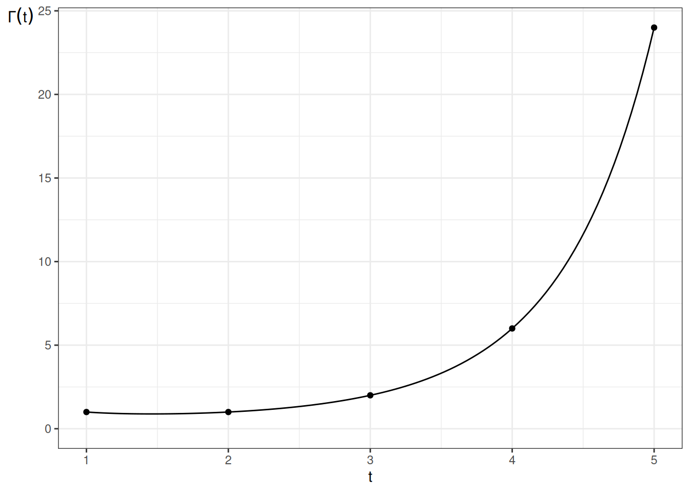
• \(\Gamma(t) \stackrel{\text{def}}{=}\int_{u=0}^{\infty}u^{t-1}\text{e}^{-u}du\)

• \(\Gamma(t) = (t-1)!\) for integers \(t \in \mathbb Z\)

• It is implemented by the gamma() function in R.

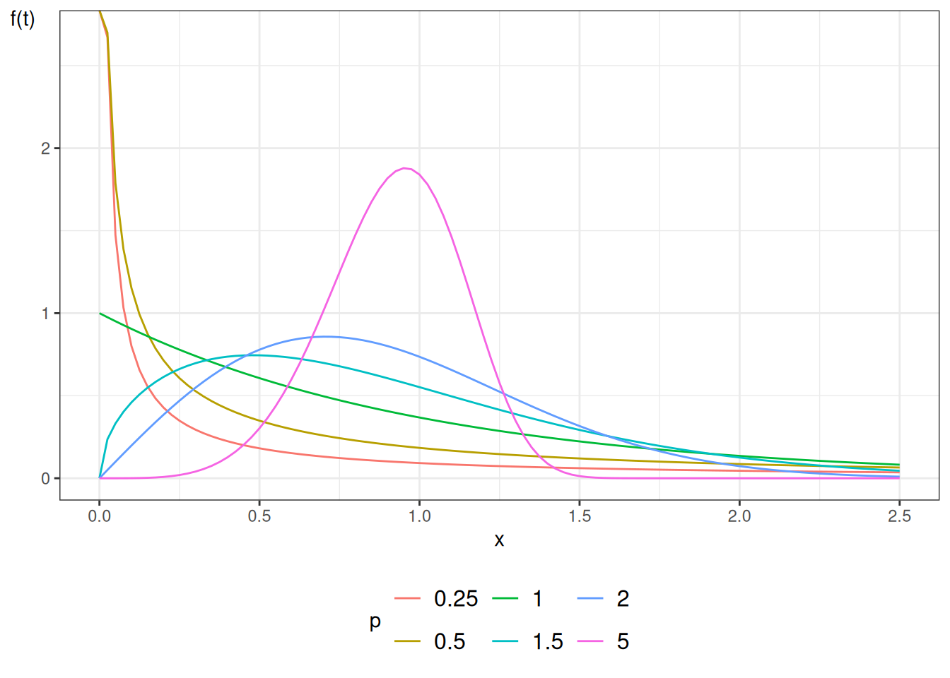
Here are some Weibull density functions, with \(\lambda = 1\) and \(p\) varying:

library(ggplot2)
lambda <- 1
ggplot() +
  geom_function(
    aes(col = "0.25"),
    fun = \(x) dweibull(x, shape = 0.25, scale = 1 / lambda)
  ) +
  geom_function(
    aes(col = "0.5"),
    fun = \(x) dweibull(x, shape = 0.5, scale = 1 / lambda)
  ) +
  geom_function(
    aes(col = "1"),
    fun = \(x) dweibull(x, shape = 1, scale = 1 / lambda)
  ) +
  geom_function(
    aes(col = "1.5"),
    fun = \(x) dweibull(x, shape = 1.5, scale = 1 / lambda)
  ) +
  geom_function(
    aes(col = "2"),
    fun = \(x) dweibull(x, shape = 2, scale = 1 / lambda)
  ) +
  geom_function(
    aes(col = "5"),
    fun = \(x) dweibull(x, shape = 5, scale = 1 / lambda)
  ) +
  theme_bw() +
  xlim(0, 2.5) +
  ylab("f(t)") +
  theme(axis.title.y = element_text(angle = 0)) +
  theme(legend.position = "bottom") +
  guides(
    col =
      guide_legend(
        title = "p",
        label.theme = element_text(size = 12)
      )
  )

Density functions for Weibull distribution

Properties of Weibull hazard functions

Theorem 1 (Properties of Weibull hazard functions) If \(T\) has a Weibull distribution, then:

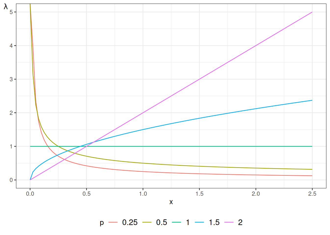
• When \(p=1\), the Weibull distribution simplifies to the exponential distribution.
• When \(p > 1\), the hazard is strictly increasing: \({\lambda}'(t) > 0\).
• When \(p < 1\), the hazard is strictly decreasing: \({\lambda}'(t) < 0\).
• \(\log{{\Lambda}(t)}\) is a straight line relative to \(\log{t}\): \(\log{{\Lambda}(t)} = p \log{\lambda} + p \log{t}\).

Proof. We prove each property of the Weibull hazard function \({\lambda}(t) = \lambda p (\lambda t)^{p-1}\):

1. Simplification to Exponential distribution when \(p=1\): Setting \(p=1\) in the Weibull hazard function yields: \[ \begin{aligned} {\lambda}(t) &= \lambda (1) (\lambda t)^{1-1} && \text{(substituting $p=1$ into Weibull hazard formula)} \\ &= \lambda \cdot 1 \cdot (\lambda t)^0 && \text{(simplifying exponent $1-1 = 0$)} \\ &= \lambda && \text{(since $(\lambda t)^0 = 1$ for $t > 0$)} \end{aligned} \] This constant value is the hazard function of the exponential distribution with parameter \(\lambda\).

2. Increasing hazard when \(p > 1\): Differentiating \({\lambda}(t) = \lambda^p p t^{p-1}\) with respect to \(t\) gives: \[ \begin{aligned} {\lambda}'(t) &\stackrel{\text{def}}{=}\frac{\partial}{\partial t} \left( \lambda^p p t^{p-1} \right) && \text{(definition of hazard derivative)} \\ &= \lambda^p p (p-1) t^{p-2} && \text{(applying power rule of differentiation)} \end{aligned} \] Since \(\lambda > 0\), \(p > 0\), and \(t > 0\), the sign of \({\lambda}'(t)\) depends entirely on the factor \((p-1)\). When \(p > 1\), \((p-1) > 0\), so \({\lambda}'(t) > 0\) for all \(t > 0\), meaning the hazard function is strictly increasing over time.

3. Decreasing hazard when \(p < 1\): Using the derivative \({\lambda}'(t) = \lambda^p p (p-1) t^{p-2}\): When \(p < 1\), \((p-1) < 0\), so \({\lambda}'(t) < 0\) for all \(t > 0\), meaning the hazard function is strictly decreasing over time.

4. Linear relationship between \(\log {\Lambda}(t)\) and \(\log t\): Taking the natural logarithm of the cumulative hazard function \({\Lambda}(t) = (\lambda t)^p\): \[ \begin{aligned} \operatorname{log}\mathopen{}\left\{{\Lambda}(t)\right\}\mathclose{} &\stackrel{\text{def}}{=}\operatorname{log}\mathopen{}\left\{(\lambda t)^p\right\}\mathclose{} && \text{(substituting Weibull cumulative hazard)} \\ &= p \operatorname{log}\mathopen{}\left\{\lambda t\right\}\mathclose{} && \text{(applying logarithm exponent rule $\log(a^b) = b \log a$)} \\ &= p \operatorname{log}\mathopen{}\left\{\lambda\right\}\mathclose{} + p \operatorname{log}\mathopen{}\left\{t\right\}\mathclose{} && \text{(applying logarithm product rule $\log(ab) = \log a + \log b$)} \end{aligned} \] Defining \(y \stackrel{\text{def}}{=}\operatorname{log}\mathopen{}\left\{{\Lambda}(t)\right\}\mathclose{}\) and \(x \stackrel{\text{def}}{=}\operatorname{log}\mathopen{}\left\{t\right\}\mathclose{}\), this equation takes the linear form \(y = a + b x\) with intercept \(a = p \operatorname{log}\mathopen{}\left\{\lambda\right\}\mathclose{}\) and slope \(b = p\).

Example 1 (Evaluating Weibull hazard shapes under different shape parameters) Consider a clinical trial evaluating time to relapse in months following cancer treatment, modeled using a Weibull distribution with scale parameter \(\lambda = 0.1\). We evaluate the hazard rate \({\lambda}(t)\) at months \(t = 1, 6, 12\) under three distinct shape parameters:

1. Decreasing hazard (\(p = 0.5\)): The hazard rate formula gives: \[ {\lambda}(t) = (0.1)(0.5)(0.1 t)^{-0.5} = \frac{0.05}{\sqrt{0.1 t}} \]

   • At \(t = 1\) month: \({\lambda}(1) = \frac{0.05}{\sqrt{0.1}} \approx 0.1581\) events per month.
   • At \(t = 6\) months: \({\lambda}(6) = \frac{0.05}{\sqrt{0.6}} \approx 0.0645\) events per month.
   • At \(t = 12\) months: \({\lambda}(12) = \frac{0.05}{\sqrt{1.2}} \approx 0.0456\) events per month. The risk of relapse is highest immediately following treatment and declines over time.

2. Constant hazard (\(p = 1.0\)): The hazard rate formula reduces to \({\lambda}(t) = \lambda = 0.1000\) events per month for all \(t\). The risk of relapse remains constant regardless of time elapsed.

3. Increasing hazard (\(p = 2.0\)): The hazard rate formula gives: \[ {\lambda}(t) = (0.1)(2.0)(0.1 t)^{1.0} = 0.02 t \]

   • At \(t = 1\) month: \({\lambda}(1) = 0.02(1) = 0.0200\) events per month.
   • At \(t = 6\) months: \({\lambda}(6) = 0.02(6) = 0.1200\) events per month.
   • At \(t = 12\) months: \({\lambda}(12) = 0.02(12) = 0.2400\) events per month. The risk of relapse increases linearly over time.

Exercise 1 Verify the calculations in Example 1 and explain how the shape parameter \(p\) affects cumulative hazard curves.

The Weibull distribution provides more flexibility than the exponential. Figure 1 shows some Weibull hazard functions, with \(\lambda = 1\) and \(p\) varying:

library(ggplot2)
library(eha)
lambda <- 1

ggplot() +
  geom_function(
    aes(col = "0.25"),
    fun = \(x) hweibull(x, shape = 0.25, scale = 1 / lambda)
  ) +
  geom_function(
    aes(col = "0.5"),
    fun = \(x) hweibull(x, shape = 0.5, scale = 1 / lambda)
  ) +
  geom_function(
    aes(col = "1"),
    fun = \(x) hweibull(x, shape = 1, scale = 1 / lambda)
  ) +
  geom_function(
    aes(col = "1.5"),
    fun = \(x) hweibull(x, shape = 1.5, scale = 1 / lambda)
  ) +
  geom_function(
    aes(col = "2"),
    fun = \(x) hweibull(x, shape = 2, scale = 1 / lambda)
  ) +
  theme_bw() +
  xlim(0, 2.5) +
  ylab(expr(lambda)) +
  theme(axis.title.y = element_text(angle = 0)) +
  theme(legend.position = "bottom") +
  guides(
    col =
      guide_legend(
        title = "p",
        label.theme = element_text(size = 12)
      )
  )

Figure 1: Hazard functions for Weibull distribution

library(ggplot2)
lambda <- 1

ggplot() +
  geom_function(
    aes(col = "0.25"),
    fun = pweibull,
    args = list(shape = 0.25, scale = 1 / lambda, lower.tail = FALSE)
  ) +
  geom_function(
    aes(col = "0.5"),
    fun = pweibull,
    args = list(shape = 0.5, scale = 1 / lambda, lower.tail = FALSE)
  ) +
  geom_function(
    aes(col = "1"),
    fun = pweibull,
    args = list(shape = 1, scale = 1 / lambda, lower.tail = FALSE)
  ) +
  geom_function(
    aes(col = "1.5"),
    fun = pweibull,
    args = list(shape = 1.5, scale = 1 / lambda, lower.tail = FALSE)
  ) +
  geom_function(
    aes(col = "2"),
    fun = pweibull,
    args = list(shape = 2, scale = 1 / lambda, lower.tail = FALSE)
  ) +
  theme_bw() +
  xlim(0, 2.5) +
  ylab("S(t)") +
  theme(axis.title.y = element_text(angle = 0)) +
  theme(legend.position = "bottom") +
  guides(
    col =
      guide_legend(
        title = "p",
        label.theme = element_text(size = 12)
      )
  )

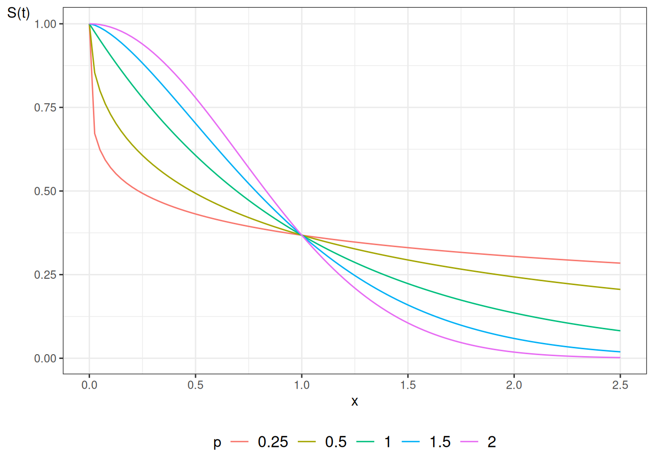
Figure 2: Survival functions for Weibull distribution

1.3 Exponential Regression

For each subject \(i\), define a linear predictor \(\eta(\tilde{x}) \stackrel{\text{def}}{=}\beta_0 + (\beta_1 x_1 + \dots + \beta_p x_p) = \tilde{x}\cdot \tilde{\beta}\). Exponential regression models the hazard rate using a log link function:

\[ \begin{aligned} {\lambda}(t \mid \tilde{x}) &\stackrel{\text{def}}{=}\operatorname{exp}\mathopen{}\left\{\eta(\tilde{x})\right\}\mathclose{} && \text{(exponential regression hazard specification)} \\ {\lambda}_0(t) &\stackrel{\text{def}}{=}{\lambda}(t \mid \tilde{0}) && \text{(baseline hazard rate definition at $\tilde{x}= \tilde{0}$)} \\ &= \operatorname{exp}\mathopen{}\left\{\eta(\tilde{0})\right\}\mathclose{} && \text{(substituting $\tilde{x}= \tilde{0}$ into hazard function)} \\ &= \operatorname{exp}\mathopen{}\left\{\beta_0 + (\beta_1 \cdot 0 + \dots + \beta_p \cdot 0)\right\}\mathclose{} && \text{(evaluating linear predictor at zero vector)} \\ &= \operatorname{exp}\mathopen{}\left\{\beta_0\right\}\mathclose{} && \text{(simplifying exponent)} \end{aligned} \]

When there are no additional predictors (\(\tilde{x}= \tilde{0}\)), the baseline hazard is constant: \(\lambda = \operatorname{exp}\mathopen{}\left\{\beta_0\right\}\mathclose{}\). This model uses a log link as in a generalized linear model for Poisson or rate outcomes. Because the hazard rate does not depend on time \(t\), the hazard ratio comparing two covariate vectors \(\tilde{x}\) and \({\tilde{x}^*}\) is constant over time:

\[ \begin{aligned} \theta_{{\lambda}}(t \mid \tilde{x}: {\tilde{x}^*}) &\stackrel{\text{def}}{=}\frac{{\lambda}(t \mid \tilde{x})}{{\lambda}(t \mid {\tilde{x}^*})} && \text{(hazard ratio definition)} \\ &= \frac{\operatorname{exp}\mathopen{}\left\{\eta(\tilde{x})\right\}\mathclose{}}{\operatorname{exp}\mathopen{}\left\{\eta({\tilde{x}^*})\right\}\mathclose{}} && \text{(substituting exponential regression hazard rates)} \\ &= \operatorname{exp}\mathopen{}\left\{\eta(\tilde{x}) - \eta({\tilde{x}^*})\right\}\mathclose{} && \text{(applying quotient rule for exponentials)} \\ &= \operatorname{exp}\mathopen{}\left\{(\tilde{x}- {\tilde{x}^*}) \cdot \tilde{\beta}\right\}\mathclose{} && \text{(expressing difference in linear predictors)} \end{aligned} \]

Thus, exponential regression models possess proportional hazards trivially.

1.4 Accelerated Failure Time

In a proportional hazards (PH) model, covariates act multiplicatively on the baseline hazard function:

\[ \begin{aligned} {\lambda}(t \mid \tilde{x}) &\stackrel{\text{def}}{=}{\lambda}_0(t) \cdot \theta_{{\lambda}}(\tilde{x}) && \text{(proportional hazards hazard rate definition)} \\ {\Lambda}(t \mid \tilde{x}) &\stackrel{\text{def}}{=}\int_{0}^{t} {\lambda}(u \mid \tilde{x}) du && \text{(cumulative hazard function definition)} \\ &= \int_{0}^{t} {\lambda}_0(u) \cdot \theta_{{\lambda}}(\tilde{x}) du && \text{(substituting proportional hazard rate)} \\ &= \theta_{{\lambda}}(\tilde{x}) \cdot {\Lambda}_0(t) && \text{(factoring constant hazard multiplier out of integral)} \\ \operatorname{S}(t \mid \tilde{x}) &\stackrel{\text{def}}{=}\operatorname{exp}\mathopen{}\left\{-{\Lambda}(t \mid \tilde{x})\right\}\mathclose{} && \text{(survival function in terms of cumulative hazard)} \\ &= \operatorname{exp}\mathopen{}\left\{-\theta_{{\lambda}}(\tilde{x}) \cdot {\Lambda}_0(t)\right\}\mathclose{} && \text{(substituting cumulative hazard)} \\ &= \left[ \operatorname{exp}\mathopen{}\left\{-{\Lambda}_0(t)\right\}\mathclose{} \right]^{\theta_{{\lambda}}(\tilde{x})} && \text{(applying exponent laws)} \\ &= \left[ \operatorname{S}_0(t) \right]^{\theta_{{\lambda}}(\tilde{x})} && \text{(substituting baseline survival function $\operatorname{S}_0(t)$)} \end{aligned} \]

An alternative modeling framework is the Accelerated Failure Time (AFT) model. Rather than multiplying the hazard rate, covariates accelerate or decelerate the progression of time itself:

\[ \operatorname{S}(t \mid \tilde{x}) \stackrel{\text{def}}{=}\operatorname{S}_0\left( t \cdot \theta_{{\lambda}}(\tilde{x}) \right) \]

where \(\theta_{{\lambda}}(\tilde{x}) \stackrel{\text{def}}{=}\operatorname{exp}\mathopen{}\left\{\eta(\tilde{x})\right\}\mathclose{}\), \(\eta(\tilde{x}) \stackrel{\text{def}}{=}\beta_1 x_1 + \dots + \beta_p x_p\), and \(\operatorname{S}_0(t) \stackrel{\text{def}}{=}\operatorname{P}(T \ge t \mid \tilde{x}= \tilde{0})\) is the baseline survival function.

We derive the expected survival time under the AFT model using change-of-variables integration:

\[ \begin{aligned} \operatorname{E}\mathopen{}\left[T \mid \tilde{x}\right]\mathclose{} &\stackrel{\text{def}}{=}\int_{0}^{\infty} \operatorname{S}(t \mid \tilde{x}) dt && \text{(expectation formula for non-negative random variable)} \\ &= \int_{0}^{\infty} \operatorname{S}_0\left( t \cdot \theta_{{\lambda}}(\tilde{x}) \right) dt && \text{(substituting AFT survival function)} \\ &= \int_{0}^{\infty} \operatorname{S}_0(u) \cdot \frac{du}{\theta_{{\lambda}}(\tilde{x})} && \text{(substituting $u = t \cdot \theta_{{\lambda}}(\tilde{x}) \implies dt = \frac{du}{\theta_{{\lambda}}(\tilde{x})}$)} \\ &= \theta_{{\lambda}}(\tilde{x})^{-1} \cdot \int_{0}^{\infty} \operatorname{S}_0(u) du && \text{(factoring constant $\theta_{{\lambda}}(\tilde{x})^{-1}$ out of integral)} \\ &= \theta_{{\lambda}}(\tilde{x})^{-1} \cdot \operatorname{E}\mathopen{}\left[T \mid \tilde{x}= \tilde{0}\right]\mathclose{} && \text{(substituting baseline expectation formula)} \end{aligned} \]

Thus, the mean survival time for a subject with covariates \(\tilde{x}\) equals the baseline mean survival time divided by the acceleration factor \(\theta_{{\lambda}}(\tilde{x}) = \operatorname{exp}\mathopen{}\left\{\eta(\tilde{x})\right\}\mathclose{}\).

We also derive the cumulative hazard and hazard rate functions under the AFT formulation:

\[ \begin{aligned} {\Lambda}(t \mid \tilde{x}) &\stackrel{\text{def}}{=}-\operatorname{log}\mathopen{}\left\{\operatorname{S}(t \mid \tilde{x})\right\}\mathclose{} && \text{(cumulative hazard function definition)} \\ &= -\operatorname{log}\mathopen{}\left\{\operatorname{S}_0\left( t \cdot \theta_{{\lambda}}(\tilde{x}) \right)\right\}\mathclose{} && \text{(substituting AFT survival function)} \\ &= {\Lambda}_0\left( t \cdot \theta_{{\lambda}}(\tilde{x}) \right) && \text{(substituting baseline cumulative hazard)} \\ {\lambda}(t \mid \tilde{x}) &\stackrel{\text{def}}{=}\frac{\partial}{\partial t} {\Lambda}(t \mid \tilde{x}) && \text{(hazard function definition)} \\ &= \frac{\partial}{\partial t} \left( {\Lambda}_0\left( t \cdot \theta_{{\lambda}}(\tilde{x}) \right) \right) && \text{(substituting AFT cumulative hazard)} \\ &= {\Lambda}_0'\left( t \cdot \theta_{{\lambda}}(\tilde{x}) \right) \cdot \frac{\partial}{\partial t} \left( t \cdot \theta_{{\lambda}}(\tilde{x}) \right) && \text{(applying chain rule of differentiation)} \\ &= {\lambda}_0\left( t \cdot \theta_{{\lambda}}(\tilde{x}) \right) \cdot \theta_{{\lambda}}(\tilde{x}) && \text{(since ${\Lambda}_0'(u) = {\lambda}_0(u)$)} \\ &= \theta_{{\lambda}}(\tilde{x}) \cdot {\lambda}_0\left( t \cdot \theta_{{\lambda}}(\tilde{x}) \right) && \text{(rearranging factors)} \end{aligned} \]

Relationship between PH and AFT models

If the baseline distribution is exponential with parameter \(\lambda\), substituting \(\operatorname{S}_0(t) = \operatorname{exp}\mathopen{}\left\{-\lambda t\right\}\mathclose{}\) into the AFT model yields:

\[ \begin{aligned} \operatorname{S}(t \mid \tilde{x}) &= \operatorname{exp}\mathopen{}\left\{-\lambda \cdot t \cdot \theta_{{\lambda}}(\tilde{x})\right\}\mathclose{} && \text{(substituting exponential baseline into AFT formula)} \\ &= \left[ \operatorname{exp}\mathopen{}\left\{-\lambda t\right\}\mathclose{} \right]^{\theta_{{\lambda}}(\tilde{x})} && \text{(applying exponent laws)} \\ &= \left[ \operatorname{S}_0(t) \right]^{\theta_{{\lambda}}(\tilde{x})} && \text{(substituting exponential baseline survival function)} \end{aligned} \]

This derivation demonstrates that the exponential AFT model is mathematically identical to the exponential PH model.

For a Weibull baseline distribution with scale \(\lambda\) and shape \(p\), the hazard and survival functions are \({\lambda}(t) = \lambda p (\lambda t)^{p-1}\) and \(\operatorname{S}(t) = \operatorname{exp}\mathopen{}\left\{-(\lambda t)^p\right\}\mathclose{}\). Specifying a proportional hazards model with subject-specific multiplier \(\theta_i \stackrel{\text{def}}{=}\operatorname{exp}\mathopen{}\left\{\eta_i\right\}\mathclose{}\) gives hazard rate \({\lambda}(t) = \lambda p (\lambda t)^{p-1} \theta_i\). Defining an adjusted scale parameter \(\lambda^* \stackrel{\text{def}}{=}\lambda \theta_i^{1/p}\), the resulting survival function is:

\[ \begin{aligned} \operatorname{S}^*(t) &\stackrel{\text{def}}{=}\operatorname{exp}\mathopen{}\left\{-(\lambda^* t)^p\right\}\mathclose{} && \text{(Weibull survival formula with scale parameter $\lambda^*$)} \\ &= \operatorname{exp}\mathopen{}\left\{-\left(\lambda \theta_i^{1/p} t\right)^p\right\}\mathclose{} && \text{(substituting $\lambda^* = \lambda \theta_i^{1/p}$)} \\ &= \operatorname{exp}\mathopen{}\left\{-(\lambda t)^p \cdot \theta_i\right\}\mathclose{} && \text{(simplifying exponent $\left(\theta_i^{1/p}\right)^p = \theta_i$)} \\ &= \left[ \operatorname{exp}\mathopen{}\left\{-(\lambda t)^p\right\}\mathclose{} \right]^{\theta_i} && \text{(applying exponent laws)} \\ &= \left[ \operatorname{S}_0(t) \right]^{\theta_i} && \text{(substituting baseline Weibull survival function)} \\ &= \operatorname{S}_0\left( t \cdot \theta_i^{1/p} \right) && \text{(expressing as AFT model with acceleration factor $\theta_i^{1/p}$)} \end{aligned} \]

This derivation proves that the Weibull model is simultaneously a proportional hazards model and an accelerated failure time model.

In terms of log survival time \(Y \stackrel{\text{def}}{=}\log T\), the Weibull AFT model takes a log-linear regression form:

\[ \begin{aligned} Y &= \alpha - \sigma \eta + \sigma W && \text{(log-linear AFT regression formulation)} \\ \alpha &\stackrel{\text{def}}{=}-\operatorname{log}\mathopen{}\left\{\lambda\right\}\mathclose{} && \text{(intercept parameter definition)} \\ \sigma &\stackrel{\text{def}}{=}\frac{1}{p} && \text{(scale parameter definition as inverse shape $p$)} \end{aligned} \]

where \(W\) follows the standard Gumbel (extreme value) distribution. The estimated AFT regression coefficients \(\hat{\beta}_{\text{AFT}}\) produced by R’s survreg() function relate directly to the PH regression coefficients \(\hat{\beta}_{\text{PH}}\) produced by coxph() via the identity \(\hat{\beta}_{\text{AFT}} = -\sigma \hat{\beta}_{\text{PH}}\).

The exponential and Weibull distributions are the only continuous distributions that are simultaneously proportional hazards models and accelerated failure time models. Other parametric families commonly used for survival data (log-logistic, log-normal, and generalized gamma) are AFT families rather than PH families; the log-logistic distribution is additionally a proportional-odds model.

1.5 Dataset: Leukemia treatments

To illustrate semi-parametric and parametric survival models, we analyze remission survival times from a clinical trial of 42 pediatric leukemia patients (Kalbfleisch and Prentice 2011). Half of the patients received a new therapy (6-mercaptopurine, 6-MP) and half received a standard control treatment.

The variables in this dataset include:

• survt: Remission duration in weeks (\(T\)).
• status: Relapse status (relapse = 1 or censored = 0).
• rx: Treatment assignment (new vs standard).
• sex: Patient sex (female vs male).
• surv: Survival outcome object created with Surv(time = survt, event = (status == "relapse")).

library(haven)
library(survival)
anderson <-
  paste0(
    "http://web1.sph.emory.edu/dkleinb/allDatasets",
    "/surv2datasets/anderson.dta"
  ) |>
  read_dta() |>
  mutate(
    status = status |>
      case_match(
        1 ~ "relapse",
        0 ~ "censored"
      ),
    sex = sex |>
      case_match(
        0 ~ "female",
        1 ~ "male"
      ),

    rx = rx |>
      case_match(
        0 ~ "new",
        1 ~ "standard"
      ),

    surv = Surv(time = survt, event = (status == "relapse"))
  )

print(anderson)

Cox semi-parametric model

We fit a Cox proportional hazards model comparing standard therapy to new therapy:

anderson_cox0 <- coxph(
  formula = surv ~ rx,
  data = anderson
)
summary(anderson_cox0)
#> Call:
#> coxph(formula = surv ~ rx, data = anderson)
#> 
#>   n= 42, number of events= 30 
#> 
#>             coef exp(coef) se(coef)    z Pr(>|z|)    
#> rxstandard 1.572     4.817    0.412 3.81  0.00014 ***
#> ---
#> Signif. codes:  0 '***' 0.001 '**' 0.01 '*' 0.05 '.' 0.1 ' ' 1
#> 
#>            exp(coef) exp(-coef) lower .95 upper .95
#> rxstandard      4.82      0.208      2.15      10.8
#> 
#> Concordance= 0.69  (se = 0.041 )
#> Likelihood ratio test= 16.4  on 1 df,   p=5e-05
#> Wald test            = 14.5  on 1 df,   p=1e-04
#> Score (logrank) test = 17.2  on 1 df,   p=3e-05

The estimated log hazard ratio \(\hat{\beta}_{\text{PH}}\) for standard treatment relative to new treatment is positive, indicating that standard therapy is associated with a higher hazard of relapse (shorter remission duration).

Weibull parametric model

We next fit a parametric Weibull accelerated failure time model using survreg():

anderson_weib <- survreg(
  formula = surv ~ rx,
  data = anderson,
  dist = "weibull"
)
summary(anderson_weib)
#> 
#> Call:
#> survreg(formula = surv ~ rx, data = anderson, dist = "weibull")
#>              Value Std. Error     z       p
#> (Intercept)  3.516      0.252 13.96 < 2e-16
#> rxstandard  -1.267      0.311 -4.08 4.5e-05
#> Log(scale)  -0.312      0.147 -2.12   0.034
#> 
#> Scale= 0.732 
#> 
#> Weibull distribution
#> Loglik(model)= -106.6   Loglik(intercept only)= -116.4
#>  Chisq= 19.65 on 1 degrees of freedom, p= 9.3e-06 
#> Number of Newton-Raphson Iterations: 5 
#> n= 42

In survreg(), regression parameters are reported on the log-time scale (\(Y = \log T = \alpha + \tilde{\beta}_{\text{AFT}} \tilde{x}+ \sigma W\)). The estimated coefficient \(\hat{\beta}_{\text{AFT}}\) for standard treatment is negative, indicating a reduction in log survival time (faster progression to relapse). The scale estimate \(\hat{\sigma}\) corresponds to \(1 / p\), and satisfies \(\hat{\beta}_{\text{AFT}} = -\hat{\sigma}\hat{\beta}_{\text{PH}}\).

Exponential parametric model

Setting the scale parameter to \(\sigma = 1\) (\(p = 1\)) yields the exponential parametric model:

anderson_exp <- survreg(
  formula = surv ~ rx,
  data = anderson,
  dist = "exp"
)
summary(anderson_exp)
#> 
#> Call:
#> survreg(formula = surv ~ rx, data = anderson, dist = "exp")
#>              Value Std. Error     z       p
#> (Intercept)  3.686      0.333 11.06 < 2e-16
#> rxstandard  -1.527      0.398 -3.83 0.00013
#> 
#> Scale fixed at 1 
#> 
#> Exponential distribution
#> Loglik(model)= -108.5   Loglik(intercept only)= -116.8
#>  Chisq= 16.49 on 1 degrees of freedom, p= 4.9e-05 
#> Number of Newton-Raphson Iterations: 4 
#> n= 42

In the exponential model, \(\hat{\beta}_{\text{AFT}} = -\hat{\beta}_{\text{PH}}\), so the AFT coefficient is equal in magnitude and opposite in sign to the Cox proportional hazards coefficient.

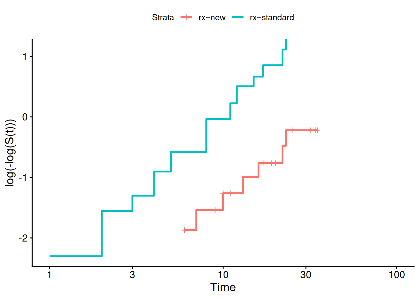
Diagnostic: complementary log-log survival plot

To check whether a Weibull proportional hazards assumption is reasonable, we inspect the complementary log-log transformation of the Kaplan-Meier survival curves, \(\log(-\log \mathop{\hat{\operatorname{S}}}\nolimits(t)) = p \log \lambda + p \log t\):

library(survminer)
survfit(
  formula = surv ~ rx,
  data = anderson
) |>
  ggsurvplot(fun = "cloglog")

Complementary log-log survival curves by treatment group

If the complementary log-log curves are approximately linear and parallel across treatment groups, then a Weibull proportional hazards model is appropriate.

2 Combining left-truncation and interval-censoring

In observational studies and clinical trials, complex observation schemes can introduce both left-truncation (delayed entry) and interval-censoring. Left-truncation occurs when subjects enter the risk set only after surviving past an entry time \(L_{\text{entry}} > 0\). Interval-censoring occurs when the exact event time \(T_i\) is unknown, but is known to fall within an interval \((L_i, R_i]\).

Standard software tools in R make distinct trade-offs between these two observation mechanisms:

coxph does left truncation but not left (or interval) censoring; survreg does interval censoring but not left truncation (or time dependent covariates).

— Terry Therneau, R-help, August 31, 2015

In particular, coxph() constructs risk sets dynamically at each observed failure time \(t_j\) using counting process format (time1 = entry, time2 = exit), enabling seamless handling of left-truncation. However, because partial likelihood relies on ordered exact failure times, standard Cox models cannot easily accommodate interval-censored data.

Conversely, survreg() accommodates interval-censored outcomes via Surv(time1 = L, time2 = R, type = "interval") by maximizing the interval parametric likelihood \(\operatorname{P}(L_i < T_i \le R_i) = \operatorname{F}_0(R_i) - \operatorname{F}_0(L_i)\). However, standard survreg() assumes all subjects enter observation at time 0, and does not condition likelihood terms on surviving past a delayed entry time \(L_{\text{entry}}\).

When a study contains both delayed entry and interval-censored event times, specialized tooling is needed. Of the packages below, only flexsurv handles both features together; the other two are listed because they cover interval censoring well and are the usual starting points, not because they solve the truncation half:

• flexsurv: Fits flexible parametric survival models and allows custom likelihood specifications that incorporate both left-truncation conditioning and interval-censored bounds.
• icenReg: Fits regression models for interval-censored data: Cox proportional-hazards, proportional-odds, and accelerated failure time. Semi-parametric and fully parametric forms are both available, but the fully parametric option covers the AFT models only. It does not itself provide left-truncation conditioning.
• interval: Fits nonparametric survival curves (NPMLE) for interval-censored data and provides weighted logrank and Wilcoxon-type tests (Fay and Shaw 2010). It is nonparametric throughout, so it supports neither regression nor truncation.

Fay, Michael P., and Pamela A. Shaw. 2010. “Exact and Asymptotic Weighted Logrank Tests for Interval Censored Data: The interval R Package.” Journal of Statistical Software 36 (2): 1–34. https://doi.org/10.18637/jss.v036.i02.

Kalbfleisch, John D, and Ross L Prentice. 2011. The Statistical Analysis of Failure Time Data. John Wiley & Sons.