Bayesian Inference

Configuring R

Functions from these packages will be used throughout this document:

library(conflicted) # check for conflicting function definitions
# library(printr) # inserts help-file output into markdown output
library(rmarkdown) # Convert R Markdown documents into a variety of formats.
library(pander) # format tables for markdown
library(ggplot2) # graphics
library(ggfortify) # help with graphics
library(dplyr) # manipulate data
library(tibble) # `tibble`s extend `data.frame`s
library(magrittr) # `%>%` and other additional piping tools
library(haven) # import Stata files
library(knitr) # format R output for markdown
library(tidyr) # Tools to help to create tidy data
library(plotly) # interactive graphics
library(dobson) # datasets from Dobson and Barnett 2018
library(parameters) # format model output tables for markdown
library(haven) # import Stata files
library(latex2exp) # use LaTeX in R code (for figures and tables)
library(fs) # filesystem path manipulations
library(survival) # survival analysis
library(survminer) # survival analysis graphics
library(KMsurv) # datasets from Klein and Moeschberger
library(parameters) # format model output tables for
library(webshot2) # convert interactive content to static for pdf
library(forcats) # functions for categorical variables ("factors")
library(stringr) # functions for dealing with strings
library(lubridate) # functions for dealing with dates and times
library(broom) # Summarizes key information about statistical objects in tidy tibbles
library(broom.helpers) # Provides suite of functions to work with regression model 'broom::tidy()' tibbles

Here are some R settings I use in this document:

rm(list = ls()) # delete any data that's already loaded into R

conflicts_prefer(dplyr::filter)
ggplot2::theme_set(
  ggplot2::theme_bw() + 
        # ggplot2::labs(col = "") +
    ggplot2::theme(
      legend.position = "bottom",
      text = ggplot2::element_text(size = 12, family = "serif")))

knitr::opts_chunk$set(message = FALSE)
options('digits' = 6)

panderOptions("big.mark", ",")
pander::panderOptions("table.emphasize.rownames", FALSE)
pander::panderOptions("table.split.table", Inf)
conflicts_prefer(dplyr::filter) # use the `filter()` function from dplyr() by default
legend_text_size = 9
run_graphs = TRUE

This appendix introduces the Bayesian approach to statistical inference, developing it from foundational principles through computational methods to fully worked analyses on real regression models. The material is organized in three parts, reflecting how students learn Bayesian reasoning:

Part 1: Foundational Theory (Section 1 through Section 4) establishes the conceptual framework. We contrast the frequentist and Bayesian paradigms, state Bayes’ theorem as an inference rule for parameters, discuss prior specification and its role, and outline hierarchical models that allow parameters to borrow strength across groups. This part mirrors (Dobson and Barnett 2018, chap. 12).

Part 2: Computational Methods (Section 5 through Section 8) explains why and how we compute with MCMC. Most real-world posteriors lack closed form, so we need simulation; we introduce Monte Carlo integration and Markov chains, describe the Metropolis-Hastings and Gibbs samplers, detail convergence diagnostics, and present model-comparison criteria. This part mirrors (Dobson and Barnett 2018, chap. 13).

Part 3: Applications (Section 9 onward) applies theory and computation to regression models we have already met in the frequentist setting — binary outcomes, survival times, random effects, and model selection via Bayesian model averaging. Throughout, we use JAGS (“Just Another Gibbs Sampler”) via R to fit models and sample posteriors. This part mirrors (Dobson and Barnett 2018, chap. 14).

1 Frequentist and Bayesian paradigms

Throughout these notes we have treated an unknown parameter \(\theta\) as a fixed but unknown constant, and we have quantified uncertainty using the sampling distribution of an estimator \(\hat\theta\) — that is, the distribution of \(\hat\theta\) over hypothetical repetitions of the data-generating process. This stance is the frequentist paradigm: probability describes long-run frequencies, and a parameter, being a constant, has no probability distribution.

The Bayesian paradigm instead treats the unknown parameter as a random variable with its own probability distribution (Dobson and Barnett 2018, chap. 12, p. 271). Probability here measures degree of belief: before seeing data we encode our uncertainty about \(\theta\) in a prior distribution \(p(\theta)\), and after observing data \(\tilde{y}\) we update that belief to a posterior distribution \(p(\theta \mid \tilde{y})\). All Bayesian inference flows from this single posterior distribution.

The two paradigms answer subtly different questions. A frequentist asks, “for what parameter values would these data be unsurprising?”; a Bayesian asks, “given these data, what should I now believe about the parameter?”. Neither question is wrong; they are different, and they call for different machinery.

1.1 Two readings of an interval estimate

The distinction is sharpest in how each paradigm interprets an interval estimate (Dobson and Barnett 2018, chap. 12, p. 271). A frequentist \(95\%\) confidence interval \(\mathopen{}\left(l(\tilde{y}),\, r(\tilde{y})\right)\mathclose{}\) is a random interval whose coverage — the probability, over repeated sampling, that the interval contains the fixed true \(\theta\) — is \(0.95\). For one realized data set the interval either contains \(\theta\) or it does not; the \(0.95\) refers to the procedure, not to the particular interval.

A Bayesian credible interval makes the statement many users want to make about a confidence interval but cannot:

Definition 1 (Credible interval) A \(100(1-\alpha)\%\) credible interval for \(\theta\) is an interval \(\mathopen{}\left(l(\tilde{y}),\, r(\tilde{y})\right)\mathclose{}\) such that, under the posterior distribution,

\[ p\mathopen{}\left[l(\tilde{y}) \le \theta \le r(\tilde{y}) \mid \tilde{y}\right]\mathclose{} \stackrel{\text{def}}{=}1 - \alpha. \]

Here the data \(\tilde{y}\) are fixed at their observed values and \(\theta\) is random, so the probability statement is about \(\theta\) directly.

2 Bayes’ theorem for parameters

The engine of Bayesian inference is Bayes’ theorem, applied to the parameter and the data. Writing \(p(\theta)\) for the prior and \(\mathcal{L}(\theta) = p(\tilde{y}\mid \theta)\) for the likelihood, the posterior is

Definition 2 (Posterior distribution) \[ p(\theta \mid \tilde{y}) \stackrel{\text{def}}{=} \frac{p(\tilde{y}\mid \theta)\,p(\theta)}{p(\tilde{y})}, \qquad p(\tilde{y}) = \int p(\tilde{y}\mid \theta)\,p(\theta)\,d\theta. \tag{1}\]

The denominator \(p(\tilde{y})\) — the marginal likelihood or evidence — does not depend on \(\theta\); it is the constant that makes the posterior integrate to one. Consequently the posterior is determined up to proportionality by the numerator alone (Dobson and Barnett 2018, chap. 12, p. 272):

\[ \underbrace{p(\theta \mid \tilde{y})}_{\text{posterior}} \;\propto\; \underbrace{p(\tilde{y}\mid \theta)}_{\text{likelihood}} \cdot \underbrace{p(\theta)}_{\text{prior}}. \tag{2}\]

This proportionality is the workhorse of applied Bayesian analysis: it lets us recognize the posterior from the shape of \(\text{likelihood} \times \text{prior}\) without ever computing the integral \(p(\tilde{y})\), and it is what makes the simulation methods of Section 5 possible.

2.1 A Gaussian mean with a Gaussian prior

When prior and likelihood combine to give a posterior in the same family as the prior, the prior is called conjugate. The normal-mean model is the cleanest example.

Example 1 (Posterior for a normal mean) Suppose \(X_1, \ldots, X_n \ \sim_{\operatorname{iid}}\ \operatorname{N}\mathopen{}\left(\mu, 1\right)\mathclose{}\) with the variance known, and place a \(\operatorname{N}\mathopen{}\left(0, 1\right)\mathclose{}\) prior on the mean: \(M \sim \operatorname{N}\mathopen{}\left(0, 1\right)\mathclose{}\). Collecting the terms of \(p(M = \mu \mid X = x) \propto p(X = x \mid M = \mu)\,p(M = \mu)\) that involve \(\mu\) and completing the square:

\[ \begin{aligned} p(M=\mu \mid X=x) &\propto p(X=x \mid M=\mu)\, p(M=\mu)\\ &\propto \operatorname{exp}\mathopen{}\left\{-\frac{1}{2}\mathopen{}\left(n\mu^2 - 2\mu n\bar{x}\right)\mathclose{}\right\}\mathclose{} \cdot \operatorname{exp}\mathopen{}\left\{-\frac{1}{2}\mu^2\right\}\mathclose{}\\ &= \operatorname{exp}\mathopen{}\left\{-\frac{1}{2}\mathopen{}\left((n+1)\mu^2 - 2\mu n\bar{x}\right)\mathclose{}\right\}\mathclose{}\\ &\propto \operatorname{exp}\mathopen{}\left\{-\frac{1}{2}(n+1)\mathopen{}\left(\mu - \frac{n}{n+1}\bar{x}\right)\mathclose{}^2\right\}\mathclose{}. \end{aligned} \]

The last line is the kernel of a normal density, so the posterior is

\[ M \mid X = x \;\sim\; \operatorname{N}\mathopen{}\left(\frac{n}{n+1}\bar{x},\; \frac{1}{n+1}\right)\mathclose{}. \]

The posterior mean \(\frac{n}{n+1}\bar{x}\) is the sample mean shrunk toward the prior mean \(0\), and the shrinkage vanishes as \(n \to \infty\).

2.2 The parameter space

Because the Bayesian treats \(\theta\) as random, the prior and posterior are distributions over the parameter space \(\Theta\) — the set of values \(\theta\) can take (Dobson and Barnett 2018, chap. 12, p. 274). The parameter space must be respected when choosing a prior: a probability \(\pi \in (0,1)\) calls for a prior supported on the unit interval (such as a Beta distribution), a variance \(\sigma^2 > 0\) calls for a prior on the positive half-line, and a vector of regression coefficients calls for a multivariate prior on \(\mathbb{R}^p\). A prior that places no mass on part of \(\Theta\) forces the posterior to do the same, no matter what the data say — so the support of the prior is itself a modeling assumption.

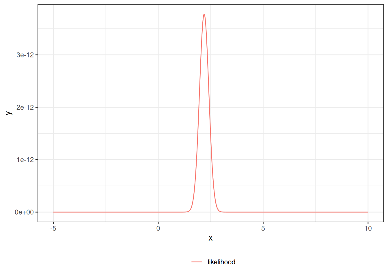
Example 2 (Credible vs. confidence interval for a normal mean) We compare the two interval estimates from Section 1.1 on simulated data from the model of Example 1. First, the frequentist interval:

set.seed(1)
mu <- 2
sigma <- 1
n <- 20
x <- rnorm(n = n, mean = mu, sd = sigma)
xbar <- mean(x)
se <- sigma / sqrt(n)
CI_freq <- xbar + se * qnorm(c(.025, .975))
print(CI_freq)
#> [1] 1.75226 2.62879

The likelihood as a function of \(\mu\):

lik <- function(mu) {
  (2 * pi * sigma^2)^(-n / 2) *
    exp(
      -1 / (2 * sigma^2) *
        (sum(x^2) - 2 * mu * sum(x) + n * (mu^2))
    )
}
ngraph <- 1001
plot1 <- ggplot() +
  geom_function(fun = lik, aes(col = "likelihood"), n = ngraph) +
  xlim(c(-5, 10)) +
  theme_bw() +
  labs(col = "") +
  theme(legend.position = "bottom")
print(plot1)

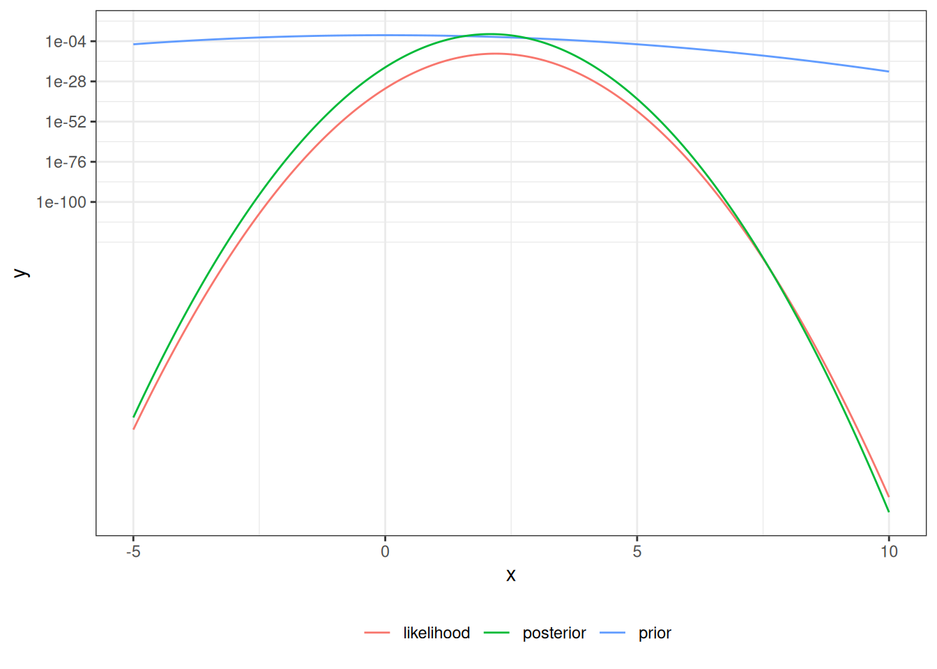
Next, the Bayesian credible interval, using the closed-form posterior \(\operatorname{N}\mathopen{}\left(\frac{n}{n+1}\bar{x},\, (n+1)^{-1}\right)\mathclose{}\) from Example 1:

mu_prior_mean <- 0
mu_prior_sd <- 1
mu_post_mean <- n / (n + 1) * xbar
mu_post_var <- 1 / (n + 1)
mu_post_sd <- sqrt(mu_post_var)
CI_bayes <- qnorm(
  p = c(.025, .975),
  mean = mu_post_mean,
  sd = mu_post_sd
)
print(CI_bayes)
#> [1] 1.65851 2.51391
prior <- function(mu) dnorm(mu, mean = mu_prior_mean, sd = mu_prior_sd)
posterior <- function(mu) dnorm(mu, mean = mu_post_mean, sd = mu_post_sd)
plot2 <- plot1 +
  geom_function(fun = prior, aes(col = "prior"), n = ngraph) +
  geom_function(fun = posterior, aes(col = "posterior"), n = ngraph)
print(plot2 + scale_y_log10())

Finally, the quantity a credible interval reports — the posterior probability that \(M\) lies in the frequentist interval — is well defined for the Bayesian but not for the frequentist:

pr_in_CI <- pnorm(
  CI_freq,
  mean = mu_post_mean,
  sd = mu_post_sd
) |> diff()
print(pr_in_CI)
#> [1] 0.930583

3 Priors

The prior distribution \(p(\theta)\) encodes what is known about \(\theta\) before the current data are seen. Choosing it is the step that most distinguishes Bayesian practice from frequentist practice, and it is where most of the controversy and most of the craft live (Dobson and Barnett 2018, chap. 12, p. 281).

3.1 Conjugate priors

A prior is conjugate to a likelihood when the resulting posterior belongs to the same parametric family as the prior. Conjugate priors make the posterior available in closed form, as in Example 1. The Beta family is conjugate to the Bernoulli/binomial likelihood:

Example 3 (Beta-Bernoulli updating) Let \(Y_1, \ldots, Y_n \ \sim_{\operatorname{iid}}\ \operatorname{Bernoulli}(\pi)\) with \(r = \sum_i y_i\) successes, and place a \(\operatorname{Beta}(a, b)\) prior on \(\pi\). By Equation 2,

\[ p(\pi \mid \tilde{y}) \propto \underbrace{\pi^{r}(1-\pi)^{n-r}}_{\text{likelihood}} \cdot \underbrace{\pi^{a-1}(1-\pi)^{b-1}}_{\text{prior}} = \pi^{a + r - 1}(1-\pi)^{b + n - r - 1}, \]

which is the kernel of a \(\operatorname{Beta}(a + r,\; b + n - r)\) density. The prior parameters \(a\) and \(b\) act as pseudo-counts of prior successes and failures: the posterior simply adds the observed \(r\) successes and \(n - r\) failures to them. With a uniform \(\operatorname{Beta}(1, 1)\) prior, \(n = 91\), and \(r = 55\), the posterior is \(\operatorname{Beta}(56, 37)\):

a_prior <- 1
b_prior <- 1
n_obs <- 91
r_obs <- 55
a_post <- a_prior + r_obs
b_post <- b_prior + n_obs - r_obs
round(c(
  post_mean = a_post / (a_post + b_post),
  post_lower = qbeta(0.025, a_post, b_post),
  post_upper = qbeta(0.975, a_post, b_post)
), 4)
#>  post_mean post_lower post_upper 
#>     0.6022     0.5014     0.6988

3.2 Informative, weakly informative, and flat priors

Priors range along a spectrum of how much they constrain \(\theta\) (Dobson and Barnett 2018, chap. 12, p. 281):

• An informative prior concentrates mass in a region supported by external knowledge (previous studies, biological limits, expert judgment). It pulls the posterior toward that region, most strongly when the data are sparse.
• A weakly informative prior rules out implausible values (for example, an odds ratio of \(10^6\)) while remaining flat across the range of scientifically plausible values.
• A flat (or noninformative) prior aims to “let the data speak,” approximating constant density over \(\Theta\). Flat priors can be improper (not integrating to one) and are not invariant to reparameterization, so they require care.

3.3 A skeptical prior

A useful special case is a skeptical prior, centered on “no effect” and deliberately tight, used to ask how strong the data must be to overturn a default of no effect (Dobson and Barnett 2018, chap. 12, p. 281).

Example 4 (A skeptical prior for a normal mean) Reusing the normal-mean model of Example 1 but with a skeptical \(\operatorname{N}\mathopen{}\left(0, \tau^2\right)\mathclose{}\) prior of standard deviation \(\tau\), the posterior mean is the precision-weighted average

\[ \operatorname{E}\mathopen{}\left[M \mid X = x\right]\mathclose{} = \frac{n\,\bar{x}}{n + 1/\tau^2}, \]

which shrinks toward \(0\) more aggressively as the prior becomes more skeptical (smaller \(\tau\)). We tabulate the posterior mean across a range of prior skepticism, holding the data fixed:

xbar_obs <- 2
n_obs2 <- 20
tau_grid <- c(0.1, 0.25, 0.5, 1, 2, 10)
post_mean <- (n_obs2 * xbar_obs) / (n_obs2 + 1 / tau_grid^2)
round(
  data.frame(prior_sd = tau_grid, posterior_mean = post_mean),
  3
)

A very skeptical prior (\(\tau = 0.1\)) drags the posterior mean almost to zero despite \(\bar{x} = 2\); a diffuse prior (\(\tau = 10\)) leaves it essentially at the sample mean.

4 Distributions and hierarchies

Many models have parameters that are themselves naturally described by a distribution with further unknown parameters (Dobson and Barnett 2018, chap. 12, p. 281). A hierarchical (or multilevel) model builds the prior in stages: a hyperprior governs hyperparameters, which govern the group-level parameters, which govern the data.

For example, with groups \(j = 1, \ldots, J\), each with its own mean \(\theta_j\), a two-level model might specify

\[ \begin{aligned} Y_{ij} \mid \theta_j &\sim \operatorname{N}\mathopen{}\left(\theta_j,\, \sigma^2\right)\mathclose{},\\ \theta_j \mid \mu, \tau &\sim \operatorname{N}\mathopen{}\left(\mu,\, \tau^2\right)\mathclose{},\\ \mu, \tau &\sim \text{hyperprior}. \end{aligned} \]

The middle level lets the groups borrow strength from one another: the posterior for each \(\theta_j\) is pulled toward the overall mean \(\mu\), by an amount governed by the between-group spread \(\tau\) that the data themselves estimate. This random-effects (multilevel) model structure is the same one fit by maximum likelihood in (Dobson and Barnett 2018, chap. 11); the Bayesian inference method differs only in placing a hyperprior on \(\mu\) and \(\tau\) and returning a full posterior for them, rather than point estimates of the variance components. Section 12 fits the same structure by simulation.

5 Foundations of MCMC

When the posterior distribution has a known closed form, we can sample from it directly and compute summaries analytically. In most real-world models, however, the normalizing constant \(p(\tilde{y})\) is intractable, making direct sampling and closed-form summaries impossible. Markov Chain Monte Carlo (MCMC) methods provide a practical solution: instead of sampling independent draws from the exact posterior, they generate a correlated sequence of draws whose long-run distribution converges to the posterior (Dobson and Barnett 2018, chap. 13, p. 287).

5.1 Why the normalizing constant is computationally challenging

The posterior is \(p(\tilde{\theta}\mid \tilde{y}) \propto p(\tilde{y}\mid \tilde{\theta})\, p(\tilde{\theta})\). The normalizing constant is

\[p(\tilde{y}) = \int p(\tilde{y}\mid \tilde{\theta})\, p(\tilde{\theta})\, d\tilde{\theta},\]

a high-dimensional integral that typically has no closed form. Computing it numerically becomes infeasible as the dimension of \(\tilde{\theta}\) grows (Dobson and Barnett 2018, chap. 13, p. 287).

MCMC sidesteps this problem: many algorithms require only the ratio \(p(\tilde{\theta}^* \mid \tilde{y}) / p(\tilde{\theta}\mid \tilde{y})\), in which the normalizing constant cancels.

5.2 Monte Carlo integration

Before introducing Markov chains, it helps to understand Monte Carlo integration (Dobson and Barnett 2018, chap. 13, p. 290). If we could draw \(M\) independent samples \(\tilde{\theta}^{(1)}, \ldots, \tilde{\theta}^{(M)} \ \sim_{\operatorname{iid}}\ p(\tilde{\theta}\mid \tilde{y})\), we could approximate any posterior expectation:

\[\operatorname{E}\mathopen{}\left[g(\tilde{\theta}) \mid \tilde{y}\right]\mathclose{} \approx \frac{1}{M} \sum_{m=1}^{M} g\!\left(\tilde{\theta}^{(m)}\right).\]

In particular, the posterior mean, posterior variance, and credible-interval endpoints are all special cases of this formula.

Example 5 (Monte Carlo posterior summaries for a Bernoulli model) Recall the Beta-Bernoulli model of Example 3, with \(n = 91\) observations and \(r = 55\) successes. The posterior is \(\pi \mid \tilde{y}\sim \operatorname{Beta}(56, 37)\). We draw \(M = 5{,}000\) samples and compare Monte Carlo summaries with exact values.

set.seed(42)
n_obs <- 91L
r_obs <- 55L
a_post <- 1L + r_obs
b_post <- 1L + n_obs - r_obs
M <- 5000L
pi_mc <- rbeta(n = M, shape1 = a_post, shape2 = b_post)
round(c(
  exact_mean  = a_post / (a_post + b_post),
  mc_mean     = mean(pi_mc),
  exact_lower = qbeta(0.025, a_post, b_post),
  mc_lower    = unname(quantile(pi_mc, 0.025)),
  exact_upper = qbeta(0.975, a_post, b_post),
  mc_upper    = unname(quantile(pi_mc, 0.975))
), 4)
#>  exact_mean     mc_mean exact_lower    mc_lower exact_upper    mc_upper 
#>      0.6022      0.6022      0.5014      0.5011      0.6988      0.7013

5.3 Markov chains

A Markov chain is a sequence of random variables \(\tilde{\theta}^{(1)}, \tilde{\theta}^{(2)}, \ldots\) such that the distribution of \(\tilde{\theta}^{(t+1)}\) depends only on \(\tilde{\theta}^{(t)}\) (the Markov property).

Definition 3 (Markov chain) A sequence of random variables \(\tilde{\theta}^{(1)}, \tilde{\theta}^{(2)}, \ldots\) is a Markov chain if, for all \(t\),

\[p(\tilde{\theta}^{(t+1)} \mid \tilde{\theta}^{(t)}, \tilde{\theta}^{(t-1)}, \ldots, \tilde{\theta}^{(1)}) = p(\tilde{\theta}^{(t+1)} \mid \tilde{\theta}^{(t)}).\]

Under mild conditions, a Markov chain converges to a unique stationary distribution. MCMC algorithms are designed so that the stationary distribution is the target posterior \(p(\tilde{\theta}\mid \tilde{y})\) (Dobson and Barnett 2018, chap. 13, p. 291).

6 MCMC Samplers

The Metropolis–Hastings (MH) algorithm is the most general MCMC method (Dobson and Barnett 2018, chap. 13, p. 293). At each iteration \(t\):

1. Propose a new value \(\tilde{\theta}^*\) from a proposal distribution \(q(\tilde{\theta}^* \mid \tilde{\theta}^{(t)})\).
2. Compute the acceptance ratio

\[\alpha = \frac{p(\tilde{y}\mid \tilde{\theta}^*)\, p(\tilde{\theta}^*)}{p(\tilde{y}\mid \tilde{\theta}^{(t)})\, p(\tilde{\theta}^{(t)})} \cdot \frac{q(\tilde{\theta}^{(t)} \mid \tilde{\theta}^*)}{q(\tilde{\theta}^* \mid \tilde{\theta}^{(t)})}.\]

3. Accept the proposal with probability \(\min(1, \alpha)\): if accepted, set \(\tilde{\theta}^{(t+1)} = \tilde{\theta}^*\). otherwise set \(\tilde{\theta}^{(t+1)} = \tilde{\theta}^{(t)}\).

Because the normalizing constant \(p(\tilde{y})\) appears in both numerator and denominator, it cancels in the ratio, so only the unnormalized posterior is needed.

Definition 4 (Metropolis–Hastings algorithm) Given a target posterior \(p(\tilde{\theta}\mid \tilde{y}) \propto p(\tilde{y}\mid \tilde{\theta})\, p(\tilde{\theta})\) and a proposal distribution \(q(\cdot \mid \tilde{\theta})\), one step of the MH algorithm proceeds as:

1. Draw \(\tilde{\theta}^* \sim q(\cdot \mid \tilde{\theta}^{(t)})\).
2. Compute \(\alpha = \min\!\left(1,\, \frac{p(\tilde{y}\mid \tilde{\theta}^*)\, p(\tilde{\theta}^*)}{p(\tilde{y}\mid \tilde{\theta}^{(t)})\, p(\tilde{\theta}^{(t)})} \cdot \frac{q(\tilde{\theta}^{(t)} \mid \tilde{\theta}^*)}{q(\tilde{\theta}^* \mid \tilde{\theta}^{(t)})}\right)\).
3. Set \(\tilde{\theta}^{(t+1)} = \tilde{\theta}^*\) with probability \(\alpha\), else \(\tilde{\theta}^{(t+1)} = \tilde{\theta}^{(t)}\).

Example 6 (Metropolis–Hastings for a Bernoulli model) We implement the MH algorithm for the same Beta-Bernoulli model as in Example 5. We use a normal random-walk proposal \(\pi^* = \pi^{(t)} + \varepsilon\), \(\varepsilon \sim \operatorname{N}\mathopen{}\left(0, \sigma^2\right)\mathclose{}\).

log_post_unnorm <- function(pi, r, n) {
  if (pi <= 0 || pi >= 1) return(-Inf)
  r * log(pi) + (n - r) * log(1 - pi)
}

mh_bernoulli <- function(n_iter, r, n, pi_init = 0.5, sigma = 0.05) {
  chain <- numeric(n_iter)
  chain[1] <- pi_init
  for (i in seq(2, n_iter)) {
    pi_curr <- chain[i - 1]
    pi_prop <- pi_curr + rnorm(1, sd = sigma)
    log_alpha <- log_post_unnorm(pi_prop, r, n) -
      log_post_unnorm(pi_curr, r, n)
    chain[i] <- if (log(runif(1)) < log_alpha) pi_prop else pi_curr
  }
  chain
}

set.seed(1)
mh_chain <- mh_bernoulli(n_iter = 5000L, r = 55L, n = 91L)

6.1 The Gibbs sampler

The Gibbs sampler is a special case of the MH algorithm for multiparameter models (Dobson and Barnett 2018, chap. 13, p. 300). When \(\tilde{\theta}= (\theta_1, \ldots, \theta_K)\), each component is updated in turn by sampling from its full conditional distribution \(p(\theta_k \mid \theta_{-k}, \tilde{y})\), where \(\theta_{-k}\) denotes all components except \(\theta_k\). The resulting proposal is always accepted (acceptance probability 1). Gibbs sampling requires that the full conditionals are available in closed form. JAGS (Just Another Gibbs Sampler) automates this approach for a wide class of models (Dobson and Barnett 2018, chap. 13).

6.2 Burn-in

Definition 5 (burn-in) The burn-in period is the initial segment of an MCMC chain that is discarded before posterior summaries are computed. During burn-in, the chain is moving toward the stationary distribution and does not yet represent draws from the posterior (Dobson and Barnett 2018, chap. 13, p. 301).

The length of the burn-in period is chosen by inspection of trace plots. A common default is to discard the first 10–20% of iterations.

7 Checking and improving MCMC

Because MCMC chains are correlated and may take time to reach stationarity, we must assess whether the chain has converged before using it for inference (Dobson and Barnett 2018, chap. 13, p. 302).

The Gelman–Rubin potential scale reduction factor (\(\hat{R}\), also called psrf in software output) compares the between-chain and within-chain variance for each parameter. Values of \(\hat{R}\) near \(1.0\) (typically \(< 1.05\)) indicate convergence; larger values suggest the chain has not yet explored the full posterior. Trace plots — time series plots of the sampled parameter values — reveal visually whether the chain has stabilized and is mixing well (bouncing around the target region) rather than still drifting or stuck.

7.1 Comparing MCMC estimates to maximum likelihood

It is reassuring — and a useful check — that for models where both approaches apply, the posterior mean from a well-mixed MCMC chain and the maximum likelihood estimate (MLE) typically agree closely when the prior is weak and the sample size is moderate or large (Dobson and Barnett 2018, chap. 13, p. 298). Intuitively, as \(n\) grows the likelihood dominates the prior, so the posterior concentrates near the MLE, and the posterior standard deviation approaches the frequentist standard error.

Example 7 (Posterior mean vs. MLE for a Bernoulli model) For the Beta-Bernoulli model with \(r = 55\) successes in \(n = 91\) trials, the MLE is \(\hat\pi = r/n\), while the posterior mean under a uniform prior is \((r+1)/(n+2)\). The two differ only by the prior’s pseudo-counts and converge as \(n\) grows:

r_obs <- 55L
n_obs <- 91L
round(c(
  mle = r_obs / n_obs,
  posterior_mean = (r_obs + 1) / (n_obs + 2)
), 4)
#>            mle posterior_mean 
#>         0.6044         0.6022

A persistent discrepancy between the two, by contrast, is a signal worth investigating: it may reflect a genuinely informative prior, an unconverged chain, or a coding error in the model.

7.2 The importance of parameterization

How a model is written affects how well its sampler mixes (Dobson and Barnett 2018, chap. 13, p. 299). Two algebraically equivalent parameterizations of the same model can produce chains with very different autocorrelation: strong posterior correlation between parameters slows a component-wise sampler, because each update can only move one coordinate at a time along a narrow, tilted ridge.

Common remedies include centering predictors (subtracting their means) so that intercept and slope are less correlated, and reparameterizing variance components to a scale on which the posterior is more nearly symmetric. These changes leave the model’s likelihood and the scientific conclusions unchanged; they alter only the geometry the sampler must explore.

8 Deviance information criterion

To compare competing Bayesian models we need a measure that balances goodness of fit against complexity, much as Akaike’s information criterion (AIC) does for likelihood-based models. The standard MCMC-based criterion is the deviance information criterion (DIC) (Dobson and Barnett 2018, chap. 13, p. 306).

Let \(D(\tilde{\theta}) = -2 \log p(\tilde{y}\mid \tilde{\theta})\) be the deviance. Write \(\overline{D}\) for its posterior mean (estimated by averaging \(D(\tilde{\theta}^{(t)})\) over the chain) and \(D(\bar{\tilde{\theta}})\) for the deviance evaluated at the posterior mean of the parameters.

Definition 6 (Deviance information criterion) The effective number of parameters and the DIC are

\[ \begin{aligned} p_D &\stackrel{\text{def}}{=}\overline{D} - D(\bar{\tilde{\theta}}),\\ \operatorname{DIC} &\stackrel{\text{def}}{=}D(\bar{\tilde{\theta}}) + 2\,p_D = \overline{D} + p_D. \end{aligned} \]

The term \(D(\bar{\tilde{\theta}})\) rewards fit, while \(p_D\) penalizes complexity: it measures how much the deviance is reduced, on average, by letting the parameters adapt to the data. As with AIC, lower DIC is better, and only differences in DIC between models fit to the same data are meaningful. Because \(p_D\) is computed directly from the posterior draws, DIC is a convenient by-product of an MCMC run; it should nonetheless be used with care, as it can behave poorly for models with weakly identified parameters or markedly non-normal posteriors.

9 A first example: a single proportion

We begin with the simplest possible model — a single Bernoulli probability — fit with JAGS (“Just Another Gibbs Sampler”), which we drive from R. This example introduces the mechanics (specifying a model, supplying data, monitoring parameters, and inspecting draws) that the later analyses reuse.

Example 8 (Bernoulli model via JAGS) First, load required packages:

library(rjags)
library(runjags)
runjags::findJAGS()
#> [1] "/usr/bin/jags"

We’ll use a simple Bernoulli model to estimate a probability parameter using Bayesian inference.

# JAGS chain initialization function
initsfunction <- function(chain) {
  stopifnot(chain %in% (1:4)) # max 4 chains allowed
  rng_seed <- (1:4)[chain]
  rng_name <- c(
    "base::Wichmann-Hill", "base::Marsaglia-Multicarry",
    "base::Super-Duper", "base::Mersenne-Twister"
  )[chain]
  return(list(".RNG.seed" = rng_seed, ".RNG.name" = rng_name))
}

# Generate sample data
set.seed(1)
data1 <- rbinom(n = 91, size = 1, prob = .6)

# Run JAGS model
jags_post0 <- run.jags(
  n.chains = 2,
  inits = initsfunction,
  model = system.file("extdata/model.dobson.jags", package = "rme"),
  data = list(r = data1, N = length(data1)),
  monitor = "p"
)
#> Compiling rjags model...
#> Calling the simulation using the rjags method...
#> Note: the model did not require adaptation
#> Burning in the model for 4000 iterations...
#> Running the model for 10000 iterations...
#> Simulation complete
#> Calculating summary statistics...
#> Calculating the Gelman-Rubin statistic for 1 variables....
#> Finished running the simulation

The results are examined by displaying the first few posterior draws:

jags_post0$mcmc |> as.array() |> head()
#>       chain
#> iter       [,1]     [,2]
#>   5001 0.584687 0.550332
#>   5002 0.576621 0.562455
#>   5003 0.651983 0.628144
#>   5004 0.598258 0.604274
#>   5005 0.611863 0.583400
#>   5006 0.565635 0.606325

10 Binary outcomes: logistic regression

For a binary outcome \(Y_i \sim \operatorname{Bernoulli}(\pi_i)\) with \(\operatorname{logit}(\pi_i) = {\tilde{x}_i}^{\top}\tilde{\beta}\), the Bayesian analysis places a prior on the coefficient vector \(\tilde{\beta}\) — typically independent, weakly informative normals such as \(\beta_j \sim \operatorname{N}\mathopen{}\left(0, \sigma_0^2\right)\mathclose{}\) with \(\sigma_0\) large on the log-odds scale — and samples the posterior \(p(\tilde{\beta}\mid \tilde{y})\) by MCMC (Dobson and Barnett 2018, chap. 14, p. 318). The posterior draws for each \(\beta_j\) are summarized by their mean and a \(95\%\) credible interval; exponentiating gives posterior summaries for the odds ratios. Unlike the frequentist fit, no large-sample normal approximation is needed: the credible interval is read directly from the posterior quantiles, and odds ratios or other nonlinear functions of \(\tilde{\beta}\) are obtained simply by transforming the draws.

Example 9 (Bayesian logistic regression) We simulate \(N = 200\) observations from a logistic model with a single continuous predictor, intercept \(\beta_0 = -0.5\) and slope \(\beta_1 = 1.2\), then recover the coefficients by MCMC.

set.seed(2024)
N <- 200L
x <- rnorm(N)
beta0_true <- -0.5
beta1_true <- 1.2
y <- rbinom(N, size = 1, prob = plogis(beta0_true + beta1_true * x))

logistic_model <- "model {
  for (i in 1:N) {
    y[i] ~ dbern(pi[i])
    logit(pi[i]) <- beta0 + beta1 * x[i]
  }
  beta0 ~ dnorm(0, 0.01)   # weakly informative: precision 0.01 = sd 10
  beta1 ~ dnorm(0, 0.01)
  OR <- exp(beta1)         # odds ratio per unit increase in x
}"

jags_logistic <- run.jags(
  model = logistic_model,
  data = list(y = y, x = x, N = N),
  monitor = c("beta0", "beta1", "OR"),
  n.chains = 2, inits = initsfunction,  # initsfunction defined in _sec-examples-proportion.qmd
  burnin = 1000, sample = 4000, method = "rjags"
)
#> Compiling rjags model...
#> Calling the simulation using the rjags method...
#> Adapting the model for 1000 iterations...
#> Burning in the model for 1000 iterations...
#> Running the model for 4000 iterations...
#> Simulation complete
#> Calculating summary statistics...
#> Calculating the Gelman-Rubin statistic for 3 variables....
#> Note: Unable to calculate the multivariate psrf
#> Finished running the simulation
summary(jags_logistic)[, c("Mean", "Lower95", "Upper95", "psrf")] |> round(3)
#>         Mean Lower95 Upper95 psrf
#> beta0 -0.657  -0.983  -0.302    1
#> beta1  1.205   0.819   1.622    1
#> OR     3.412   2.174   4.899    1

The posterior means recover \(\beta_0 \approx -0.5\) and \(\beta_1 \approx 1.2\), each \(95\%\) credible interval covers its true value, and the convergence statistic psrf (\(\hat{R}\)) is near \(1\). The odds-ratio summary comes for free by monitoring \(\operatorname{exp}\mathopen{}\left\{(\right\}\mathclose{}\beta_1)\).

11 Survival analysis

Parametric survival models (for example, exponential or Weibull event times) admit a Bayesian treatment in which priors are placed on the baseline-hazard parameters and the regression coefficients, and the posterior is sampled by MCMC (Dobson and Barnett 2018, chap. 14, p. 330). Censoring is handled inside the model through the likelihood: an event contributes its density \({\lambda}(y)\,\operatorname{S}(y)\) and a censored observation contributes its survival probability \(\operatorname{S}(y)\), exactly as in the frequentist right-censored likelihood.

Example 10 (Bayesian exponential survival regression) We simulate right-censored exponential survival times with a binary covariate (say, treatment) whose true log hazard ratio is \(\beta_1 = -0.7\), and fit the model with the zeros trick, which lets us write the exact censored log-likelihood directly in JAGS.

set.seed(2026)
N <- 200L
x <- rbinom(N, size = 1, prob = 0.5)
beta0_true <- log(0.05)   # log baseline hazard
beta1_true <- -0.7        # log hazard ratio for x = 1
event_time <- rexp(N, rate = exp(beta0_true + beta1_true * x))
cens_time <- rexp(N, rate = 0.03)
y <- pmin(event_time, cens_time)
event <- as.integer(event_time <= cens_time)   # 1 = event, 0 = censored

surv_model <- "model {
  C <- 10000
  for (i in 1:N) {
    log(lambda[i]) <- beta0 + beta1 * x[i]
    # exponential log-likelihood, right-censored:
    loglik[i] <- event[i] * log(lambda[i]) - lambda[i] * y[i]
    phi[i] <- C - loglik[i]
    zeros[i] ~ dpois(phi[i])
  }
  beta0 ~ dnorm(0, 0.01)
  beta1 ~ dnorm(0, 0.01)
  HR <- exp(beta1)   # hazard ratio for x = 1 vs x = 0
}"

jags_surv <- run.jags(
  model = surv_model,
  data = list(y = y, x = x, event = event, N = N, zeros = rep(0, N)),
  monitor = c("beta0", "beta1", "HR"),
  n.chains = 2, inits = initsfunction,  # initsfunction defined in _sec-examples-proportion.qmd
  burnin = 1000, sample = 4000, method = "rjags"
)
#> Compiling rjags model...
#> Calling the simulation using the rjags method...
#> Adapting the model for 1000 iterations...
#> Burning in the model for 1000 iterations...
#> Running the model for 4000 iterations...
#> Simulation complete
#> Calculating summary statistics...
#> Calculating the Gelman-Rubin statistic for 3 variables....
#> Finished running the simulation
summary(jags_surv)[, c("Mean", "Lower95", "Upper95", "psrf")] |> round(3)
#>         Mean Lower95 Upper95  psrf
#> beta0 -3.115  -3.386  -2.861 1.000
#> beta1 -0.532  -0.933  -0.139 1.002
#> HR     0.600   0.374   0.843 1.002

The posterior for \(\beta_1\) concentrates near the true \(-0.7\), and the monitored \(\operatorname{exp}\mathopen{}\left\{(\right\}\mathclose{}\beta_1)\) gives the hazard ratio with a credible interval that accounts for the censoring without any large-sample approximation.

12 Random effects

The random-effects (multilevel) model structure — group-level parameters \(\theta_j \sim \operatorname{N}\mathopen{}\left(\mu, \tau^2\right)\mathclose{}\) drawn from a common distribution — is the same one fit by maximum likelihood in (Dobson and Barnett 2018, chap. 11). What changes here is the inference method: the Bayesian treatment (the hierarchical model of Section 4) places priors on the hyperparameters \(\mu\) and \(\tau\) and samples their joint posterior together with the group-level parameters. The posterior shrinks each group’s estimate toward the overall mean by an amount the data determine through \(\tau\), and — unlike the maximum-likelihood fit — the posterior for \(\tau\) propagates the uncertainty in the between-group spread into every group-level summary (Dobson and Barnett 2018, chap. 14, p. 333).

Example 11 (Bayesian random-intercept model) We simulate \(J = 8\) groups of \(12\) observations each, with group means drawn from \(\operatorname{N}\mathopen{}\left(\mu, \tau^2\right)\mathclose{}\) (\(\mu = 5\), \(\tau = 1.5\)) and within-group noise \(\sigma = 2\), then recover the hyperparameters.

set.seed(2025)
J <- 8L
n_j <- 12L
mu_true <- 5
tau_true <- 1.5
sigma_true <- 2
theta_true <- rnorm(J, mean = mu_true, sd = tau_true)
group <- rep(seq_len(J), each = n_j)
y <- rnorm(J * n_j, mean = theta_true[group], sd = sigma_true)

re_model <- "model {
  for (i in 1:N) {
    y[i] ~ dnorm(theta[group[i]], inv_sigma2)
  }
  for (j in 1:J) {
    theta[j] ~ dnorm(mu, inv_tau2)   # random intercepts
  }
  mu ~ dnorm(0, 1.0E-4)
  inv_sigma2 ~ dgamma(0.01, 0.01)
  inv_tau2 ~ dgamma(0.01, 0.01)
  sigma <- 1 / sqrt(inv_sigma2)   # within-group SD
  tau <- 1 / sqrt(inv_tau2)       # between-group SD
}"

jags_re <- run.jags(
  model = re_model,
  data = list(y = y, group = group, N = length(y), J = J),
  monitor = c("mu", "tau", "sigma"),
  n.chains = 2, inits = initsfunction,  # initsfunction defined in _sec-examples-proportion.qmd
  burnin = 1000, sample = 4000, method = "rjags"
)
#> Compiling rjags model...
#> Calling the simulation using the rjags method...
#> Note: the model did not require adaptation
#> Burning in the model for 1000 iterations...
#> Running the model for 4000 iterations...
#> Simulation complete
#> Calculating summary statistics...
#> Calculating the Gelman-Rubin statistic for 3 variables....
#> Finished running the simulation
summary(jags_re)[, c("Mean", "Lower95", "Upper95", "psrf")] |> round(3)
#>        Mean Lower95 Upper95  psrf
#> mu    5.556   4.838   6.262 1.000
#> tau   0.664   0.067   1.416 1.012
#> sigma 2.166   1.856   2.503 1.000

The posterior recovers the overall mean \(\mu \approx 5\), the between-group SD \(\tau \approx 1.5\), and the within-group SD \(\sigma \approx 2\). Crucially, the credible interval for \(\tau\) reports genuine uncertainty about the between-group spread — uncertainty a frequentist point estimate of the variance component discards.

13 Bayesian model averaging

When several candidate models are plausible, Bayesian model averaging (BMA) forms predictions by averaging over models, weighting each by its posterior probability rather than committing to a single “best” model (Dobson and Barnett 2018, chap. 14, p. 338). This propagates model uncertainty — not just parameter uncertainty — into the final inference. Unlike the single-model fits above, BMA requires fitting and comparing a collection of models and computing their posterior weights, which connects directly to the model-comparison criteria of Section 8 and to our predictor-selection chapter.

Example 12 (A BIC approximation to Bayesian model averaging) Marginal likelihoods are hard to compute, but the Bayesian information criterion provides a convenient approximation to the posterior model probability (Schwarz 1978): for model \(m\), \(p(m \mid \tilde{y}) \propto \operatorname{exp}\mathopen{}\left\{-\tfrac{1}{2}\operatorname{BIC}_m\right\}\mathclose{}\). We simulate data in which only \(x_1\) and \(x_2\) affect the outcome (with \(x_3\) irrelevant), enumerate every subset of the three predictors, and form BIC-based model weights.

set.seed(2027)
N <- 120L
x1 <- rnorm(N)
x2 <- rnorm(N)
x3 <- rnorm(N) # irrelevant
y <- 1 + 0.8 * x1 + 0.5 * x2 + rnorm(N)
dat <- data.frame(y, x1, x2, x3)

predictors <- c("x1", "x2", "x3")
subsets <- unlist(
  lapply(0:3, function(k) combn(predictors, k, simplify = FALSE)),
  recursive = FALSE
)
models <- lapply(subsets, function(vars) {
  rhs <- if (length(vars)) paste(vars, collapse = " + ") else "1"
  lm(as.formula(paste("y ~", rhs)), data = dat)
})

# BIC approximation to posterior model probabilities:
bic <- vapply(models, BIC, numeric(1))
weight <- exp(-0.5 * (bic - min(bic)))
weight <- weight / sum(weight)

The posterior inclusion probability of each predictor is the total weight of the models that contain it:

pip <- vapply(
  predictors,
  function(v) sum(weight[vapply(subsets, function(s) v %in% s, logical(1))]),
  numeric(1)
)
round(pip, 3)
#>    x1    x2    x3 
#> 1.000 1.000 0.152

and the model-averaged slope for \(x_1\) averages each model’s estimate (taken as \(0\) when \(x_1\) is absent from that model):

beta_x1 <- vapply(models, function(m) {
  cf <- coef(m)
  if ("x1" %in% names(cf)) cf[["x1"]] else 0
}, numeric(1))
round(c(bma_slope_x1 = sum(weight * beta_x1)), 3)
#> bma_slope_x1 
#>        0.947

The real predictors \(x_1\) and \(x_2\) receive inclusion probabilities near \(1\), the irrelevant \(x_3\) a small one, and the model-averaged slope for \(x_1\) sits near its true value \(0.8\) — with the averaging across models, rather than a single selected model, accounting for which predictors belong.

14 Further reading

The following resources provide deeper coverage of Bayesian inference.

14.1 UC Davis courses

• STA 015C: “Introduction to Statistical Data Science III”
• STA 035C: “Statistical Data Science III”
• STA 145: “Bayesian Statistical Inference”
• ECL 234: “Bayesian Models - A Statistical Primer”
• PLS 207: “Applied Statistical Modeling for the Environmental Sciences”
• PSC 205H: “Applied Bayesian Statistics for Social Scientists”
• POL 280: “Bayesian Methods: for Social & Behavioral Sciences”
• BAX 442: “Advanced Statistics”

14.2 Books

• Ross (2022) is a free online textbook
• “Population health thinking with Bayesian networks” (Aragon 2018) is on my to-read list
• McElreath (2020)
  • very popular recently
  • author used to be a UCD professor
  • ECL 234 uses this book
  • videos: https://www.youtube.com/playlist?list=PLDcUM9US4XdPz-KxHM4XHt7uUVGWWVSus
  • course materials: https://github.com/rmcelreath/stat_rethinking_2024
• Korner-Nievergelt and Korner-Nievergelt (2015)
• Cowles (2013)
• Kéry et al. (2012)
• Hobbs and Hooten (2015) has been used in PLS 207

References

Aragon, Tomas J. 2018. Population Health Thinking with Bayesian Networks. https://escholarship.org/uc/item/8000r5m5.

Cowles, Mary Kathryn. 2013. Applied Bayesian Statistics: With R and OpenBUGS Examples. Vol. 98. Springer Texts in Statistics. Springer Nature. https://doi.org/10.1007/978-1-4614-5696-4.

Dobson, Annette J, and Adrian G Barnett. 2018. An Introduction to Generalized Linear Models. 4th ed. CRC press. https://doi.org/10.1201/9781315182780.

Hobbs, N. Thompson, and Mevin B Hooten. 2015. Bayesian Models: A Statistical Primer for Ecologists. STU - Student edition. Princeton University Press.

Kéry, Marc., Michael. Schaub, and Steven R. Beissinger. 2012. Bayesian Population Analysis Using WinBUGS : A Hierarchical Perspective. 1st ed. Academic Press. https://shop.elsevier.com/books/bayesian-population-analysis-using-winbugs/kery/978-0-12-387020-9.

Korner-Nievergelt, Fränzi, and Fränzi Korner-Nievergelt. 2015. Bayesian Data Analysis in Ecology Using Linear Models with R, BUGS, and Stan. 1st ed. Academic Press.

McElreath, Richard. 2020. Statistical Rethinking : A Bayesian Course with Examples in R and Stan. Second edition. Chapman & Hall/CRC Texts in Statistical Science Series. CRC Press.

Ross, Kevin. 2022. An Introduction to Bayesian Reasoning and Methods. Online. https://bookdown.org/kevin_davisross/bayesian-reasoning-and-methods/.

Schwarz, Gideon. 1978. “Estimating the Dimension of a Model.” The Annals of Statistics 6 (2): 461–64. https://doi.org/10.1214/aos/1176344136.