Introduction to GLMs

1 Introduction

Configuring R

Functions from these packages will be used throughout this document:

library(conflicted) # check for conflicting function definitions
# library(printr) # inserts help-file output into markdown output
library(rmarkdown) # Convert R Markdown documents into a variety of formats.
library(pander) # format tables for markdown
library(ggplot2) # graphics
library(ggfortify) # help with graphics
library(dplyr) # manipulate data
library(tibble) # `tibble`s extend `data.frame`s
library(magrittr) # `%>%` and other additional piping tools
library(haven) # import Stata files
library(knitr) # format R output for markdown
library(tidyr) # Tools to help to create tidy data
library(plotly) # interactive graphics
library(dobson) # datasets from Dobson and Barnett 2018
library(parameters) # format model output tables for markdown
library(haven) # import Stata files
library(latex2exp) # use LaTeX in R code (for figures and tables)
library(fs) # filesystem path manipulations
library(survival) # survival analysis
library(survminer) # survival analysis graphics
library(KMsurv) # datasets from Klein and Moeschberger
library(parameters) # format model output tables for
library(webshot2) # convert interactive content to static for pdf
library(forcats) # functions for categorical variables ("factors")
library(stringr) # functions for dealing with strings
library(lubridate) # functions for dealing with dates and times
library(broom) # Summarizes key information about statistical objects in tidy tibbles
library(broom.helpers) # Provides suite of functions to work with regression model 'broom::tidy()' tibbles

Here are some R settings I use in this document:

rm(list = ls()) # delete any data that's already loaded into R

conflicts_prefer(dplyr::filter)
ggplot2::theme_set(
  ggplot2::theme_bw() + 
        # ggplot2::labs(col = "") +
    ggplot2::theme(
      legend.position = "bottom",
      text = ggplot2::element_text(size = 12, family = "serif")))

knitr::opts_chunk$set(message = FALSE)
options('digits' = 6)

panderOptions("big.mark", ",")
pander::panderOptions("table.emphasize.rownames", FALSE)
pander::panderOptions("table.split.table", Inf)
conflicts_prefer(dplyr::filter) # use the `filter()` function from dplyr() by default
legend_text_size = 9
run_graphs = TRUE

2 Welcome

Welcome to Epidemiology 204: Quantitative Epidemiology III (Statistical Models).

Epi 204 is a course on regression modeling.

3 What you should already know

Warning

Epi 202, Epi 203, and Sta 108 are prerequisites for this course. If you haven’t passed one of these courses, talk to me ASAP.

Epi 202: probability models

• Probability distributions
  • binomial
  • Poisson
  • Gaussian
  • exponential

• Characteristics of probability distributions
  • Mean, median, mode, quantiles
  • Variance, standard deviation, overdispersion

• Characteristics of samples
  • independence, dependence, covariance, correlation
  • ranks, order statistics
  • identical vs nonidentical distribution (homogeneity vs heterogeneity)
  • Laws of Large Numbers
  • Central Limit Theorem for the mean of an iid sample

Epi 203: inference for one or several homogenous populations

• the maximum likelihood inference framework:
  • likelihood functions
  • log-likelihood functions
  • score functions
  • estimating equations
  • information matrices
  • point estimates
  • standard errors
  • confidence intervals
  • hypothesis tests
  • p-values

• Hypothesis tests for one, two, and >2 groups:
  • t-tests/ANOVA for Gaussian models
  • chi-square tests for binomial and Poisson models
  • nonparametric tests:
    • Wilcoxon signed-rank test for matched pairs
    • Mann–Whitney/Kruskal-Wallis rank sum test for \(\geq 2\) independent samples
    • Fisher’s exact test for contingency tables
    • Cochran–Mantel–Haenszel-Cox log-rank test

For all of the quantities above, and especially for confidence intervals and p-values, you should know how both:

• how to compute them
• how to interpret them

Stat 108: linear regression models

• building models for Gaussian outcomes
  • multiple predictors
  • interactions
• regression diagnostics
• fundamentals of R programming; e.g.:
  • Wickham et al. (2023)
  • Dalgaard (2008)
• RMarkdown or Quarto for formatting homework
  • LaTeX for writing math in RMarkdown/Quarto

4 What we will cover in this course

• Linear (Gaussian) regression models (review and more details)

• Regression models for non-Gaussian outcomes

  • binary
  • count
  • time to event

• Statistical analysis using R

We will start where Epi 203 left off: with linear regression models.

5 Motivations for regression models

Exercise 1 Why do we need regression models?

Solution 1.

• when there’s not enough data to analyze every subgroup of interest individually

• especially when subgroups are defined using continuous predictors

5.1 Uses of regression models

Vittinghoff et al. (2012, sec. 1.3) identifies three broad motivations for using multipredictor regression models:

Multipredictor regression can be a powerful tool for addressing three important practical questions. … [These] include prediction, isolating the effect of a single predictor, and understanding multiple predictors.

1. Prediction: “Multipredictor regression is a powerful and general tool for using multiple measured predictors to make useful predictions for future observations.”

2. Isolating the Effect of a Single Predictor: “In settings where multiple, related predictors contribute to study outcomes, it will be important to consider multiple predictors even when a single predictor is of interest.” (e.g., to minimize confounding and support causal interpretation)

3. Understanding Multiple Predictors: “Multipredictor regression can also be used when our aim is to identify multiple independent predictors of a study outcome — independent in the sense that they appear to have an effect over and above other measured variables.” (including mediation and interaction)

Kleinbaum et al. (2014, sec. 4.1) provides a more granular list of eight overlapping applications of regression analysis:

In practice, a regression analysis is appropriate for several possibly overlapping situations, including the following:

1. Characterize the association: “You want to characterize the relationship between the dependent and independent variables by determining the extent, direction, and strength of the association.”

2. Prediction: “You seek a quantitative formula or equation to describe (e.g., predict) the dependent variable \(Y\) as a function of the independent variables \(X_1, X_2, \ldots, X_k\).”

3. Controlled description: “You want to describe quantitatively or qualitatively the relationship between \(X_1, X_2, \ldots, X_k\) and \(Y\) but control for the effects of still other variables \(X_{k+1}, X_{k+2}, \ldots, X_{k+p}\), which you believe have an important relationship with the dependent variable.”

4. Variable selection: “You want to determine which of several independent variables are important and which are not for describing or predicting a dependent variable. You may want to control for other variables. You may also want to rank independent variables in their order of importance.”

5. Model selection: “You want to determine the best mathematical model for describing the relationship between a dependent variable and one or more independent variables.”

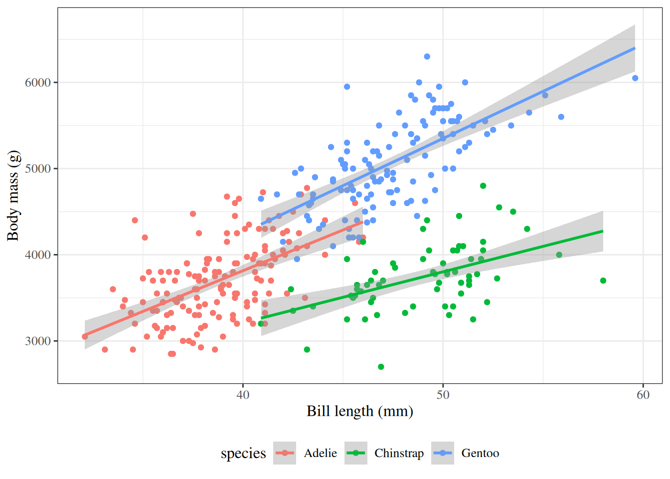
6. Comparing regression relationships: “You want to compare several derived regression relationships.” (e.g., whether a relationship between two variables differs across subgroups)

7. Interaction: “You want to assess the interactive effects of two or more independent variables with regard to a dependent variable.”

8. Adjusted coefficient estimation: “You want to obtain a valid and precise estimate of one or more regression coefficients from a larger set of regression coefficients in a given model.” (i.e., estimating the effect of one variable after adjusting for others)

Relating the two lists

The two lists use different levels of granularity to describe the same landscape of regression uses. Vittinghoff et al. (2012) provides three broad categories, while Kleinbaum et al. (2014) identifies eight more specific applications.

Table 1: Comparing the categorizations of regression model uses in Vittinghoff et al. (2012, sec. 1.3) and Kleinbaum et al. (2014, sec. 4.1)

Vittinghoff et al. (2012) category	Kleinbaum et al. (2014) application(s)
Prediction	Application 2 (prediction)
Isolating the Effect of a Single Predictor	Application 8 (adjusted coefficient estimation)
Understanding Multiple Predictors	Application 1 (characterize association), Application 3 (controlled description), Application 4 (variable selection), Application 5 (model selection), Application 6 (comparing regression relationships), Application 7 (interaction)

Applications 6 and 7 are related but distinct: Application 6 asks whether a derived regression relationship (e.g., a coefficient or the overall model) differs across pre-defined groups, typically by comparing models fit separately for each group. Application 7 asks whether two predictors interact within a single model — that is, whether the effect of one predictor on the outcome depends on the value of another predictor. In that sense, Application 6 can be viewed as a special case of Application 7 where the grouping variable is the effect modifier.

The key conceptual distinction made by Vittinghoff et al. (2012) — but not explicitly highlighted by Kleinbaum et al. (2014) — is between prediction (forecasting future outcomes) and causal inference (estimating the effect of a specific predictor). This distinction has important implications for model building strategy: prediction models can include any variables that improve predictive accuracy, while causal inference requires careful consideration of confounding, mediation, and the causal structure of the data.

Prediction, Inference, and Causal Inference

The goal of prediction is to forecast an outcome \(Y\) for new observations, given observed predictor variables \(X_1, \ldots, X_p\). In a prediction problem, the model is often treated as a “black box”: we care about predictive accuracy, not about the exact form or interpretation of the relationship between predictors and outcome (James et al. 2021, chap. 2).

Example 1 For example, a clinical prediction model might identify which patients are at highest risk of hospital readmission, using demographics, diagnoses, and laboratory values, without requiring that each predictor be causally related to readmission.

At its core, prediction aspires to minimize uncertainty: the goal is that, by including enough informative predictors and combining them flexibly, we can reduce as much as possible the residual randomness in our forecasts.

Statistical inference also studies the relationship between \(Y\) and \(X_1, \ldots, X_p\), but the goal shifts from accuracy to understanding: which predictors are associated with the response, in what direction, and by how much (James et al. 2021, chap. 2)?

Example 2 For example, a cohort study might estimate the association between smoking and lung cancer incidence, along with a confidence interval quantifying uncertainty about the magnitude of that association.

Unlike prediction, statistical inference treats the uncertainty in outcomes as a meaningful quantity to characterize, not merely residual noise to be minimized.

Causal inference asks a distinct third question. A predictive association between a predictor \(X\) and an outcome \(Y\) does not imply that intervening to change \(X\) will change \(Y\). Causal inference addresses this gap: it asks what would happen to \(Y\) if we were to actively set \(X\) to a particular value, rather than passively observe it (Vittinghoff et al. 2012, chap. 12).

Example 3 For example, even if smoking is strongly associated with lung cancer in observational data, causal inference asks whether reducing smoking rates would cause a reduction in lung cancer incidence — a question that requires additional assumptions about the data-generating process.

One useful framing of causal inference is as a prediction problem in counterfactual worlds: predicting what outcomes would have occurred under treatment conditions that were not actually administered. Under the potential outcomes framework (Neyman 1990; Rubin 1974, 688–701; Vittinghoff et al. 2012, chap. 12), individual causal effects are treated as deterministic in principle — each person has a fixed potential outcome under each treatment condition — and uncertainty arises from the fact that we can observe only one potential outcome per person, and from heterogeneity in effects across individuals.

Accurate causal inference typically requires accounting for confounding: in observational data, people who receive a treatment are often systematically different from those who do not in ways that also affect the outcome. These differences can make predictive associations misleading for causal questions.

A useful informal distinction: prediction asks which individuals are at highest risk, while causal inference asks what is the effect of a particular intervention, and statistical inference asks what the association is without necessarily specifying an intervention.

For an accessible introduction to the distinction between prediction and statistical inference, see James et al. (2021, chap. 2). For coverage of causal inference methods in an epidemiological setting, see Vittinghoff et al. (2012, chap. 12) and Hernán and Robins (2020, pt. I). For an in-depth treatment, see the causal inference chapter.

5.2 Example: Adelie penguins

Figure 1: Palmer penguins

5.3 Linear regression

ggpenguins2 <-
  ggpenguins +
  stat_smooth(
    method = "lm",
    formula = y ~ x,
    geom = "smooth"
  )

ggpenguins2 |> print()

Figure 2: Palmer penguins with linear regression fit

5.4 Curved regression lines

ggpenguins2 <- ggpenguins +
  stat_smooth(
    method = "lm",
    formula = y ~ log(x),
    geom = "smooth"
  ) +
  xlab("Bill length (mm)") +
  ylab("Body mass (g)")
ggpenguins2

Figure 3: Palmer penguins - curved regression lines

5.5 Multiple regression

ggpenguins <-
  palmerpenguins::penguins |>
  ggplot(
    aes(
      x = bill_length_mm,
      y = body_mass_g,
      color = species
    )
  ) +
  geom_point() +
  stat_smooth(
    method = "lm",
    formula = y ~ x,
    geom = "smooth"
  ) +
  xlab("Bill length (mm)") +
  ylab("Body mass (g)")
ggpenguins |> print()

Figure 4: Palmer penguins - multiple groups

5.6 Modeling non-Gaussian outcomes

library(glmx)
data(BeetleMortality)
beetles <- BeetleMortality |>
  mutate(
    pct = died / n,
    survived = n - died
  )

plot1 <-
  beetles |>
  ggplot(aes(x = dose, y = pct)) +
  geom_point(aes(size = n)) +
  xlab("Dose (log mg/L)") +
  ylab("Mortality rate (%)") +
  scale_y_continuous(labels = scales::percent) +
  # xlab(bquote(log[10]), bquote(CS[2])) +
  scale_size(range = c(1, 2))

print(plot1)

Figure 5: Mortality rates of adult flour beetles after five hours’ exposure to gaseous carbon disulphide (Bliss 1935)

5.7 Why don’t we use linear regression?

beetles_long <-
  beetles |>
  reframe(
    .by = everything(),
    outcome = c(
      rep(1, times = died),
      rep(0, times = survived)
    )
  )

lm1 <-
  beetles_long |>
  lm(
    formula = outcome ~ dose,
    data = _
  )


range1 <- range(beetles$dose) + c(-.2, .2)

f_linear <- function(x) predict(lm1, newdata = data.frame(dose = x))

plot2 <-
  plot1 +
  geom_function(fun = f_linear, aes(col = "Straight line")) +
  labs(colour = "Model", size = "")
print(plot2)

Figure 6: Mortality rates of adult flour beetles after five hours’ exposure to gaseous carbon disulphide (Bliss 1935)

5.8 Zoom out

Figure 7: Mortality rates of adult flour beetles after five hours’ exposure to gaseous carbon disulphide (Bliss 1935)

5.9 log transformation of dose?

lm2 <-
  beetles_long |>
  lm(formula = outcome ~ log(dose), data = _)

f_linearlog <- function(x) predict(lm2, newdata = data.frame(dose = x))

plot3 <- plot2 +
  expand_limits(x = c(1.6, 2)) +
  geom_function(fun = f_linearlog, aes(col = "Log-transform dose"))

print(plot3 + expand_limits(x = c(1.6, 2)))

Figure 8: Mortality rates of adult flour beetles after five hours’ exposure to gaseous carbon disulphide (Bliss 1935)

5.10 Logistic regression

glm1 <- beetles |>
  glm(formula = cbind(died, survived) ~ dose, family = "binomial")

f <- function(x) {
  glm1 |> 
    predict(newdata = data.frame(dose = x), type = "response")
}

plot4 <- plot3 + geom_function(fun = f, aes(col = "Logistic regression"))
print(plot4)

Figure 9: Mortality rates of adult flour beetles after five hours’ exposure to gaseous carbon disulphide (Bliss 1935)

6 Structure of regression models

Exercise 2 What is a regression model?

Definition 1 (Regression model) Regression models are conditional probability distribution models:

\[\operatorname{P}(Y|\tilde{X})\]

Exercise 3 What are some of the names used for the variables in a regression model \(\operatorname{P}(Y|\tilde{X})\)?

Definition 2 (Outcome) The outcome variable in a regression model is the variable whose distribution is being described; in other words, the variable on the left-hand side of the “|” (“pipe”) symbol.

The outcome variable is also called the response variable, regressand, predicted variable, explained variable, experimental variable, output variable, dependent variable, endogenous variables, target, or label.

and is typically denoted \(Y\).

Definition 3 (Predictors) The predictor variables in a regression model are the conditioning variables defining subpopulations among which the outcome distribution might vary.

Predictors are also called regressors, covariates, independent variables, explanatory variables, risk factors, exposure variables, input variables, exogenous variables, candidate variables (Dunn and Smyth (2018)), carriers (Dunn and Smyth (2018)), manipulated variables, or features and are typically denoted \(\tilde{X}\). ¹

1. The “~” (“tilde”) symbol in the notation \(\tilde{X}\) indicates that \(\tilde{X}\) is a vector. See the appendices for a table of notation used in these notes.

Table 2: Common pairings of terms for variables \(\tilde{X}\) and \(Y\) in regression models \(P(Y|\tilde{X})\) ¹

\(\tilde{X}\)	\(Y\)	usual context
input	output
independent	dependent
predictor	predicted or response
explanatory	explained
exogenous	endogenous	econometrics
manipulated	measured	randomized controlled experiments
exposure	outcome	epidemiology
feature	label or target	machine learning

1. adapted from https://en.wikipedia.org/wiki/Dependent_and_independent_variables#Synonyms

Exercise 4 What is the general structure of a generalized linear model?

Solution 2. Generalized linear models have three components:

1. The outcome distribution family: \(\operatorname{p}(Y|\mu(\tilde{x}))\)

2. The link function: \(g(\mu(\tilde{x})) = \eta(\tilde{x})\)

3. The linear component: \(\eta(\tilde{x}) = \tilde{x}\cdot \beta\)

---

1. The outcome distribution family (a.k.a. the random component of the model)

• Gaussian (normal)
• Binomial
• Poisson
• Exponential
• Gamma
• Negative binomial

---

2. The linear component (a.k.a. the linear predictor or linear functional form) describing how the covariates combine to define subpopulations:

\[\eta(\tilde{x}) \stackrel{\text{def}}{=}\tilde{x}^{\top} \tilde{\beta}= \beta_0 + \beta_1 x_1 + \beta_2 x_2 + ...\]

---

3. The link function relating the outcome distribution to the linear component, typically through the mean:

• identity: \(\mu(y) = \eta(\tilde{x})\)
• logit: \(\operatorname{log}\mathopen{}\left\{\frac{\mu(y)}{1-\mu(y)}\right\}\mathclose{} = \eta(\tilde{x})\)
• log: \(\operatorname{log}\mathopen{}\left\{\mu(y)\right\}\mathclose{} = \eta(\tilde{x})\)
• inverse: \(\mathopen{}\left(\mu(y)\right)^{-1}\mathclose{} = \eta(\tilde{x})\)
• clog-log: \(\operatorname{log}\mathopen{}\left\{-\operatorname{log}\mathopen{}\left\{1-\mu(y)\right\}\mathclose{}\right\}\mathclose{} = \eta(\tilde{x})\)

Components 2 and 3 together are sometimes called the systematic component of the model (for example, in Dunn and Smyth (2018)).

Exercises

Exercise 5 (Identifying GLM components) (adapted from Dobson and Barnett (2018), Chapter 4, and Dunn and Smyth (2018), Chapter 5)

For each of the following scenarios, identify the three components of the GLM: (1) the outcome distribution, (2) the link function \(g(\cdot)\), and (3) the linear predictor \(\eta = \tilde{x}\cdot \tilde{\beta}\).

(a) Modeling the probability of a binary outcome (disease/no disease) as a function of continuous predictors, using the logit link.

(b) Modeling count data (number of events per person-year) as a function of continuous predictors, using the log link.

(c) Modeling a continuous, strictly positive outcome using a gamma distribution and log link.

Solution. (a) Logistic regression:

1. Outcome distribution: \(Y_i \mid \tilde{x}_i \ \sim_{\perp\!\!\!\perp}\ \text{Bernoulli}(\pi_i)\)
2. Link function: logit link, \(g(\pi) = \operatorname{log}\mathopen{}\left\{\pi/(1-\pi)\right\}\mathclose{}\)
3. Linear predictor: \(\eta_i = \beta_0 + \beta_1 x_{i1} + \cdots + \beta_p x_{ip}\)

The mean function (inverse link) is: \(\pi_i = \operatorname{expit}(\eta_i) = \frac{e^{\eta_i}}{1 + e^{\eta_i}}\).

(b) Poisson (log-linear) regression:

1. Outcome distribution: \(Y_i \mid \tilde{x}_i \ \sim_{\perp\!\!\!\perp}\ \operatorname{Pois}(\mu_i)\)
2. Link function: log link, \(g(\mu) = \operatorname{log}\mathopen{}\left\{\mu\right\}\mathclose{}\)
3. Linear predictor: \(\eta_i = \beta_0 + \beta_1 x_{i1} + \cdots + \beta_p x_{ip}\)

The mean function (inverse link) is: \(\mu_i = e^{\eta_i}\).

(c) Gamma regression with log link:

1. Outcome distribution: \(Y_i \mid \tilde{x}_i \ \sim_{\perp\!\!\!\perp}\ \text{Gamma}(\text{mean} = \mu_i)\)
2. Link function: log link, \(g(\mu) = \operatorname{log}\mathopen{}\left\{\mu\right\}\mathclose{}\)
3. Linear predictor: \(\eta_i = \beta_0 + \beta_1 x_{i1} + \cdots + \beta_p x_{ip}\)

The mean function is: \(\mu_i = e^{\eta_i}\).

References

Dalgaard, Peter. 2008. Introductory Statistics with r. New York, NY: Springer New York. https://link.springer.com/book/10.1007/978-0-387-79054-1.

Dobson, Annette J, and Adrian G Barnett. 2018. An Introduction to Generalized Linear Models. 4th ed. CRC press. https://doi.org/10.1201/9781315182780.

Dunn, Peter K, and Gordon K Smyth. 2018. Generalized Linear Models with Examples in R. Vol. 53. Springer. https://link.springer.com/book/10.1007/978-1-4419-0118-7.

Hernán, Miguel A., and James M. Robins. 2020. Causal Inference: What If. Chapman & Hall/CRC. https://www.hsph.harvard.edu/miguel-hernan/causal-inference-book/.

James, Gareth, Daniela Witten, Trevor Hastie, and Robert Tibshirani. 2021. An Introduction to Statistical Learning: With Applications in R. 2nd ed. Springer. https://doi.org/10.1007/978-1-0716-1418-1.

Kleinbaum, David G, Lawrence L Kupper, Azhar Nizam, K Muller, and ES Rosenberg. 2014. Applied Regression Analysis and Other Multivariable Methods. 5th ed. Cengage Learning. https://www.cengage.com/c/applied-regression-analysis-and-other-multivariable-methods-5e-kleinbaum/9781285051086/.

Neyman, Jerzy. 1990. “On the Application of Probability Theory to Agricultural Experiments. Essay on Principles. Section 9.” Statistical Science 5 (4): 465–72. https://doi.org/10.1214/ss/1177012031.

Rubin, Donald B. 1974. “Estimating Causal Effects of Treatments in Randomized and Nonrandomized Studies.” Journal of Educational Psychology 66 (5): 688–701. https://doi.org/10.1037/h0037350.

Vittinghoff, Eric, David V Glidden, Stephen C Shiboski, and Charles E McCulloch. 2012. Regression Methods in Biostatistics: Linear, Logistic, Survival, and Repeated Measures Models. 2nd ed. Springer. https://doi.org/10.1007/978-1-4614-1353-0.

Wickham, Hadley, Mine Çetinkaya-Rundel, and Garrett Grolemund. 2023. R for Data Science. " O’Reilly Media, Inc.". https://r4ds.hadley.nz/.