Causal Inference

Estimating causal effects from regression models

Configuring R

Functions from these packages will be used throughout this document:

library(conflicted) # check for conflicting function definitions
# library(printr) # inserts help-file output into markdown output
library(rmarkdown) # Convert R Markdown documents into a variety of formats.
library(pander) # format tables for markdown
library(ggplot2) # graphics
library(ggfortify) # help with graphics
library(dplyr) # manipulate data
library(tibble) # `tibble`s extend `data.frame`s
library(magrittr) # `%>%` and other additional piping tools
library(haven) # import Stata files
library(knitr) # format R output for markdown
library(tidyr) # Tools to help to create tidy data
library(plotly) # interactive graphics
library(dobson) # datasets from Dobson and Barnett 2018
library(parameters) # format model output tables for markdown
library(haven) # import Stata files
library(latex2exp) # use LaTeX in R code (for figures and tables)
library(fs) # filesystem path manipulations
library(survival) # survival analysis
library(survminer) # survival analysis graphics
library(KMsurv) # datasets from Klein and Moeschberger
library(parameters) # format model output tables for
library(webshot2) # convert interactive content to static for pdf
library(forcats) # functions for categorical variables ("factors")
library(stringr) # functions for dealing with strings
library(lubridate) # functions for dealing with dates and times
library(broom) # Summarizes key information about statistical objects in tidy tibbles
library(broom.helpers) # Provides suite of functions to work with regression model 'broom::tidy()' tibbles

Here are some R settings I use in this document:

rm(list = ls()) # delete any data that's already loaded into R

conflicts_prefer(dplyr::filter)
ggplot2::theme_set(
  ggplot2::theme_bw() + 
        # ggplot2::labs(col = "") +
    ggplot2::theme(
      legend.position = "bottom",
      text = ggplot2::element_text(size = 12, family = "serif")))

knitr::opts_chunk$set(message = FALSE)
options('digits' = 6)

panderOptions("big.mark", ",")
pander::panderOptions("table.emphasize.rownames", FALSE)
pander::panderOptions("table.split.table", Inf)
conflicts_prefer(dplyr::filter) # use the `filter()` function from dplyr() by default
legend_text_size = 9
run_graphs = TRUE

Acknowledgements

This chapter is adapted from (Vittinghoff et al. 2012, chap. 9) and draws on the companion causal inference notes available at https://d-morrison.github.io/cie/.

See also Hernán and Robins (2020) for a comprehensive treatment of causal inference from observational data.

1 Introduction

Regression models describe statistical associations between variables. But in many research settings, the goal is not merely to describe associations but to estimate causal effects: what would happen if we intervened to change a variable?

“No causes in, no causes out.” (Holland 1986)

A statistical model alone cannot tell us whether an observed association is causal or spurious. Causal inference requires additional assumptions — about the data-generating process — that must be justified using subject-matter knowledge.

The causal inference framework covered in this chapter is based on the potential outcomes model (Rubin 1974; Holland 1986). This framework provides:

• A precise language for defining causal effects
• Explicit assumptions required to identify causal effects from data
• Estimation methods that target specific causal estimands

For more resources on causal inference, including additional courses and books, see https://d-morrison.github.io/cie/.

2 Potential Outcomes

Causal inference is about estimating the effect of interventions — what would happen if we changed something? Statistical associations alone do not answer causal questions.

The fundamental challenge in causal inference is that we can only observe one potential outcome for each unit: the outcome under the treatment that actually occurred. This is called the fundamental problem of causal inference (Holland 1986).

Definition 1 (Potential outcomes) For a binary treatment \(A \in \{0, 1\}\), the potential outcomes for unit \(i\) are:

• \(Y_i(1)\): the outcome that would be observed if unit \(i\) received treatment (\(A_i = 1\))
• \(Y_i(0)\): the outcome that would be observed if unit \(i\) received control (\(A_i = 0\))

These are also called counterfactual outcomes, because for each unit, one of them is necessarily counterfactual (it corresponds to a treatment that did not occur).

Definition 2 (Observed outcome) The observed outcome for unit \(i\) is the potential outcome corresponding to the treatment actually received: \[Y_i = Y_i(A_i) = A_i \cdot Y_i(1) + (1 - A_i) \cdot Y_i(0)\]

This is sometimes called the consistency assumption: the observed outcome under the observed treatment equals the potential outcome under that treatment.

Definition 3 (Individual causal effect) The individual causal effect for unit \(i\) is the difference between that unit’s two potential outcomes: \[\tau_i = Y_i(1) - Y_i(0)\]

Because of the fundamental problem of causal inference, we can never observe both \(Y_i(1)\) and \(Y_i(0)\) for the same unit, so individual causal effects are generally not identified.

3 Causal Estimands

Since individual causal effects are not identified, causal inference focuses on population-level causal estimands: averages of potential outcomes over a population.

Definition 4 (Average Treatment Effect (ATE)) The Average Treatment Effect is the expected difference in potential outcomes in the study population: \[\text{ATE} = \text{E}{\left[Y(1) - Y(0)\right]} = \text{E}{\left[Y(1)\right]} - \text{E}{\left[Y(0)\right]}\]

The ATE represents the average causal effect of treatment compared with control, averaged over all units in the population (both those who would and would not actually receive treatment).

Definition 5 (Average Treatment Effect on the Treated (ATT)) The Average Treatment Effect on the Treated is the expected difference in potential outcomes among units who actually received treatment: \[\text{ATT} = \text{E}{\left[Y(1) - Y(0) \mid A = 1\right]} = \text{E}{\left[Y(1) \mid A = 1\right]} - \text{E}{\left[Y(0) \mid A = 1\right]}\]

The ATT answers the question: “On average, how much did treatment help the people who received it?”

Definition 6 (Average Treatment Effect on the Untreated (ATU)) The Average Treatment Effect on the Untreated is the expected difference in potential outcomes among units who did not receive treatment: \[\text{ATU} = \text{E}{\left[Y(1) - Y(0) \mid A = 0\right]} = \text{E}{\left[Y(1) \mid A = 0\right]} - \text{E}{\left[Y(0) \mid A = 0\right]}\]

The ATU answers the question: “On average, how much would treatment have helped the people who did not receive it?”

The ATE, ATT, and ATU are equal when treatment assignment is independent of potential outcomes (e.g., in a perfectly conducted randomized trial): \[\text{ATE} = \text{ATT} = \text{ATU} \quad \text{when } A \perp\!\!\!\perp (Y(0), Y(1))\]

In observational studies, these three estimands can differ substantially. The choice of estimand depends on the research question.

4 Causal Assumptions

Three key assumptions are required to identify causal effects from observed data (Hernán and Robins 2020):

4.1 Consistency

Definition 7 (Consistency) The consistency assumption states that the observed outcome for a treated unit equals that unit’s potential outcome under treatment, and similarly for control: \[Y_i = Y_i(A_i)\]

Consistency requires that the treatment is well-defined: there is only one version of treatment, or different versions have the same effect on the outcome. Violations of consistency (e.g., different doses of a drug being lumped together as “treated”) can introduce bias.

4.2 Exchangeability (No Unmeasured Confounding)

Definition 8 (Exchangeability) Exchangeability (also called no unmeasured confounding or ignorability) states that, conditional on observed covariates \(\tilde{L}\), treatment assignment is independent of potential outcomes: \[A \perp\!\!\!\perp (Y(0), Y(1)) \mid \tilde{L}\]

Intuitively, this means that among individuals with the same covariate values, treatment was assigned as if at random — there are no unmeasured common causes of treatment and outcome.

Unconditional exchangeability (\(A \perp\!\!\!\perp (Y(0), Y(1))\)) holds in perfectly randomized trials. Conditional exchangeability requires adjusting for \(\tilde{L}\).

4.3 Positivity

Definition 9 (Positivity) The positivity assumption states that every individual has a positive probability of receiving each treatment level, conditional on their covariate values: \[0 < \text{P}{A = 1 \mid \tilde{L} = \tilde{l}} < 1 \quad \text{for all } \tilde{l} \text{ in the support of } \tilde{L}\]

Without positivity, some subgroups have no treated (or untreated) members, making it impossible to estimate the counterfactual outcome for those subgroups. This is sometimes called the positivity violation or practical positivity violation when near-zero probabilities occur in small strata.

These three assumptions — consistency, exchangeability, and positivity — are collectively sufficient to identify causal effects from observed data. They are sometimes summarized as “no interference, no unmeasured confounders, no positivity violations.”

These assumptions are untestable from the data alone; they must be justified using subject-matter knowledge.

5 Randomized Experiments

In a randomized controlled trial (RCT), treatment is assigned by the investigator using a random mechanism, independent of any characteristics of the participants. This makes the treatment groups exchangeable: the distribution of potential outcomes is the same in treated and untreated groups.

As a result, in a perfectly randomized trial:

\[\text{E}{\left[Y(1)\right]} = \text{E}{\left[Y \mid A = 1\right]} \quad \text{and} \quad \text{E}{\left[Y(0)\right]} = \text{E}{\left[Y \mid A = 0\right]}\]

The observed mean difference between treatment groups is an unbiased estimate of the ATE:

\[\widehat{\text{ATE}} = \bar{Y}_{A=1} - \bar{Y}_{A=0}\]

Randomization achieves unconditional exchangeability: \(A \perp\!\!\!\perp (Y(0), Y(1))\). Because there are no common causes of treatment assignment and the outcome, there is no confounding. The observed association between \(A\) and \(Y\) in the data is a direct measure of the causal effect.

5.1 The HERS study: a randomized trial example

The “heart and estrogen/progestin study” (HERS) was a clinical trial of hormone therapy for prevention of recurrent heart attacks and death among 2,763 post-menopausal women with existing coronary heart disease (CHD) (Hulley et al. 1998).

The trial was conducted at 20 US clinical centers. Participants were randomized to receive either conjugated equine estrogens (0.625 mg/day) plus medroxyprogesterone acetate (2.5 mg/day) or a matching placebo (Hulley et al. 1998). Women were followed for an average of 4.1 years (Hulley et al. 1998).

The primary outcome was nonfatal myocardial infarction or CHD death (Hulley et al. 1998).

In HERS, hormone therapy (HT) was randomized, so the treatment groups were exchangeable at baseline. The observed difference in CHD event rates between the HT and placebo groups estimates the causal effect of HT.

Despite observational studies suggesting up to 35–80% fewer recurrent CHD events among hormone users than non-users, (Hulley et al. 1998), HERS found no significant difference in CHD event rates between the hormone therapy (HT) and placebo groups (relative hazard 0.99; 95% CI: 0.80–1.22) (Hulley et al. 1998).

The HERS investigators noted a statistically significant time trend: more CHD events occurred in the HT group in year 1, while fewer occurred in years 4 and 5, suggesting that HT may have early harmful effects that are later reversed.

A key finding was that HT significantly altered lipid profiles:

• LDL cholesterol: 11% lower in the HT group (Hulley et al. 1998).
• HDL cholesterol: 10% higher in the HT group (Hulley et al. 1998).

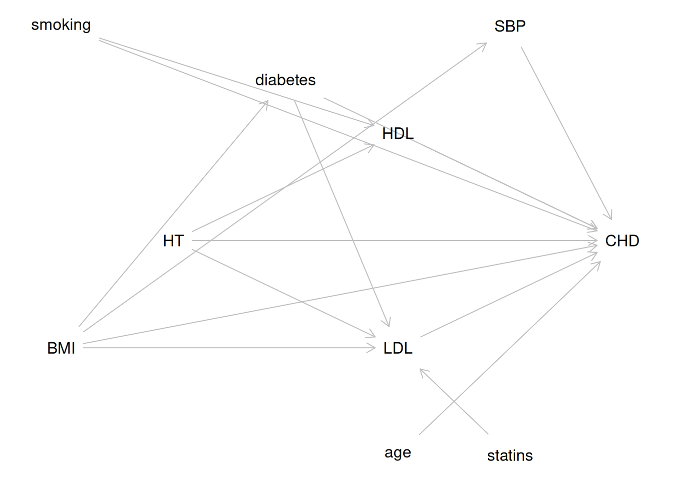
Yet these favorable lipid changes did not translate into fewer CHD events overall. One explanation consistent with the DAG in Figure 1 is that the effects of HT on lipids (a mediator pathway) were offset by other, harmful pathways — possibly thrombotic — that are not captured in the lipid mediators.

Hulley et al. (1998) also noted that HT increased the rate of venous thromboembolic events (relative hazard 2.89; 95% CI: 1.50–5.58) and gallbladder disease (relative hazard 1.38; 95% CI: 1.00–1.92).

The HERS result illustrates the gap between observational evidence and causal evidence: prior observational studies had suggested large benefits of HT, but these reflected confounding by the “healthy user” effect — women who voluntarily used HT tended to be healthier overall. Randomization in HERS removed this confounding.

5.2 Covariate adjustment in RCTs

Although randomization ensures no confounding, adjusting for baseline covariates in an RCT can still be useful:

• Improved precision: Adjusting for strong predictors of the outcome reduces residual variance and narrows confidence intervals.
• Covariate imbalance: When randomization produces chance imbalances in small trials, adjustment can correct for these.

However, in an RCT, covariates that are mediators of the treatment effect (i.e., variables affected by treatment) should generally not be adjusted for when estimating the total causal effect of treatment. Adjusting for mediators blocks part of the causal pathway and gives only the direct effect of treatment.

6 Observational Studies

In an observational study, treatment is not assigned by the investigator. Instead, individuals self-select into treatment, or treatment is assigned based on clinical or administrative criteria. As a result, treatment groups may differ systematically in ways that also affect the outcome — this is called confounding.

6.1 Confounding

Definition 10 (Confounding) Confounding occurs when there is a common cause of both the treatment \(A\) and the outcome \(Y\). This common cause is called a confounder.

In the potential outcomes framework, confounding means that treatment assignment is not independent of potential outcomes: \[A \not\perp\!\!\!\perp (Y(0), Y(1))\]

As a result, the observed association between \(A\) and \(Y\) does not equal the causal effect of \(A\) on \(Y\).

Directed Acyclic Graphs (DAGs) provide a formal graphical tool for representing causal assumptions and identifying confounders, mediators, colliders, and sufficient adjustment sets.

6.2 Directed Acyclic Graphs (DAGs)

A Directed Acyclic Graph (DAG) is a graphical model that encodes assumed causal relationships among variables.

In a DAG:

• Nodes represent variables.
• Directed edges (arrows) represent direct causal effects.
• The graph is acyclic: there are no directed cycles (a variable cannot cause itself, even indirectly).

DAGs are used in causal inference to:

• Identify confounders that must be adjusted for.
• Identify mediators that should generally not be adjusted for when estimating the total causal effect.
• Identify colliders that should not be adjusted for (adjusting for a collider opens a non-causal path).

6.3 Key concepts from DAG theory

Definition 11 (Confounder) A confounder of the relationship between an exposure \(X\) and outcome \(Y\) is a variable \(C\) that is a common cause of both \(X\) and \(Y\). By contrast, a mediator lies on the causal path from \(X\) to \(Y\) and is not a common cause of \(X\) and \(Y\).

Adjusting for confounders removes confounding bias.

Definition 12 (Mediator) A mediator \(M\) is a variable that lies on the causal pathway from the exposure \(X\) to the outcome \(Y\): \[X \to M \to Y\]

Adjusting for a mediator blocks the indirect causal pathway through \(M\), so the estimated coefficient for \(X\) reflects only the direct effect of \(X\) on \(Y\) not through \(M\).

Whether to adjust for mediators depends on the research question:

• If you want the total causal effect of \(X\) on \(Y\), do not adjust for \(M\).
• If you want the direct effect of \(X\) on \(Y\) not through \(M\), adjust for \(M\).

Definition 13 (Collider) A collider is a variable \(L\) that is caused by two or more variables on a path: \[X \to L \leftarrow Y\]

Adjusting for a collider opens a non-causal (backdoor) path between \(X\) and \(Y\), introducing collider bias.

Definition 14 (Backdoor criterion) A set of variables \(\tilde{L}\) satisfies the backdoor criterion with respect to the ordered pair \((A, Y)\) in a DAG if:

1. No variable in \(\tilde{L}\) is a descendant of \(A\).
2. \(\tilde{L}\) blocks every path between \(A\) and \(Y\) that has an arrow into \(A\) (a “backdoor” path).

If \(\tilde{L}\) satisfies the backdoor criterion, then adjusting for \(\tilde{L}\) identifies the causal effect of \(A\) on \(Y\): \[\text{E}{\left[Y(a)\right]} = \sum_{\tilde{l}} \text{E}{\left[Y \mid A = a, \tilde{L} = \tilde{l}\right]} \text{P}{\tilde{L} = \tilde{l}}\]

6.4 HERS study DAG

The “heart and estrogen/progestin study” (HERS) was a clinical trial of hormone therapy for prevention of recurrent heart attacks and death among 2,763 post-menopausal women with existing coronary heart disease (CHD) (Hulley et al. 1998).

The trial was conducted at 20 US clinical centers. Participants were randomized to receive either conjugated equine estrogens (0.625 mg/day) plus medroxyprogesterone acetate (2.5 mg/day) or a matching placebo (Hulley et al. 1998). Women were followed for an average of 4.1 years (Hulley et al. 1998).

The primary outcome was nonfatal myocardial infarction or CHD death (Hulley et al. 1998).

We now examine the assumed causal structure among key baseline variables, treatment, and recurrent CHD events.

Figure 1 shows a DAG for the HERS study, representing the assumed causal structure among key variables.

The main goal of the HERS study was to estimate the causal effect of hormone therapy (HT) on recurrent CHD event risk.

Table 1

Data dictionary for key HERS variables used in the DAG and examples.

Variable	Meaning	Type
HT	Hormone-therapy assignment (placebo vs estrogen+progestin)	Binary categorical
CHD	Recurrent coronary heart disease event outcome	Binary categorical
age	Baseline age (years)	Continuous
smoking	Baseline smoking status	Binary categorical
diabetes	Baseline diabetes status	Binary categorical
BMI	Body mass index	Continuous
LDL	Low-density lipoprotein cholesterol	Continuous
HDL	High-density lipoprotein cholesterol	Continuous
statins	Baseline statin use	Binary categorical
SBP	Systolic blood pressure	Continuous

library(dagitty)

hers_dag <- dagitty(
  'dag {
    HT [exposure, pos="0,0"]
    CHD [outcome, pos="4,0"]
    age [pos="2,2"]
    smoking [pos="-1,-2"]
    diabetes [pos="1,-1.5"]
    BMI [pos="-1,1"]
    LDL [pos="2,1"]
    HDL [pos="2,-1"]
    statins [pos="3,2"]
    SBP [pos="3,-2"]

    HT -> CHD
    HT -> HDL
    HT -> LDL
    age -> CHD
    smoking -> CHD
    smoking -> HDL
    BMI -> CHD
    BMI -> diabetes
    BMI -> SBP
    BMI -> LDL
    diabetes -> CHD
    diabetes -> LDL
    LDL -> CHD
    HDL -> CHD
    statins -> LDL
    SBP -> CHD
  }'
)

plot(hers_dag)

Figure 1: Directed Acyclic Graph (DAG) for the HERS study. HT = hormone therapy (exposure); CHD = recurrent coronary heart disease events (outcome); HDL = high-density lipoprotein; LDL = low-density lipoprotein; SBP = systolic blood pressure.

In Figure 1:

• age is prognostic for CHD: older women are at higher risk of CHD events. Since HT was randomized in HERS, age is not a confounder of the HT → CHD relationship, but adjusting for age can improve precision.
• LDL and HDL are mediators: hormone therapy affects lipid levels, which in turn affect CHD risk.
• BMI is a common cause of diabetes, SBP, and LDL.
• statins (statin use) affects LDL independently of HT (statins are medications prescribed to lower LDL).
• This DAG is simplified; a more complete model might include additional variables such as anti-hypertensive medication use.

6.5 What variables should we adjust for?

Using DAG theory, we can identify the minimum adjustment set needed to estimate the total causal effect of HT on CHD.

Table 2

adjustmentSets(
  hers_dag,
  exposure = "HT",
  outcome = "CHD",
  type = "minimal"
)
#>  {}

Since HT was randomized in HERS, there are no backdoor paths from HT to CHD. The adjustmentSets() function confirms that no adjustment is needed to estimate the total causal effect of HT on CHD.

The variables LDL and HDL are mediators on the path HT → LDL/HDL → CHD, so they should not be included when estimating the total causal effect of HT on CHD.

Including LDL and HDL in the model would block a part of the causal effect of HT, giving us only the direct effect of HT on CHD (not through lipids).

6.6 Analyzing LDL in the HERS study

The HERS baseline dataset includes LDL and HDL cholesterol, allowing us to examine the effect of hormone therapy on lipid levels.

Here we build models to predict LDL cholesterol, illustrating how DAG thinking guides predictor selection.

library(haven)
library(dplyr)

hers <- read_stata(fs::path_package("rme", "extdata/hersdata.dta"))

hers_ldl <-
  hers |>
  filter(!is.na(LDL)) |>
  mutate(
    HT = factor(HT, levels = c(0, 1), labels = c("Placebo", "HT")),
    statins = factor(statins, levels = c(0, 1), labels = c("No", "Yes")),
    diabetes = factor(diabetes, levels = c(0, 1), labels = c("No", "Yes")),
    smoking = factor(smoking, levels = c(0, 1), labels = c("No", "Yes"))
  )

library(gtsummary)

hers_ldl |>
  dplyr::select(LDL, HT, age, BMI, diabetes, smoking, statins) |>
  tbl_summary(by = HT) |>
  add_overall() |>
  bold_labels()

Table 3: Summary table for LDL analysis variables in HERS

Characteristic	Overall N = 2,7521	Placebo N = 1,3791	HT N = 1,3731
LDL cholesterol (mg/dl)	141 (120, 166)	141 (119, 165)	141 (120, 167)
age in years	67 (62, 72)	68 (62, 72)	67 (62, 72)
BMI (kg/m^2)	27.7 (24.6, 31.7)	27.6 (24.5, 31.7)	27.9 (24.7, 31.8)
Unknown	5	4	1
diabetes	727 (26%)	350 (25%)	377 (27%)
smoking	355 (13%)	180 (13%)	175 (13%)
statins	998 (36%)	516 (37%)	482 (35%)
1 Median (Q1, Q3); n (%)

Unadjusted model

model_ldl_unadj <-
  lm(LDL ~ HT, data = hers_ldl)

model_ldl_unadj |>
  tbl_regression() |>
  bold_labels()

Table 4: Unadjusted linear regression for LDL in HERS

Characteristic	Beta	95% CI	p-value
HT
Placebo	—	—
HT	0.36	-2.5, 3.2	0.8
Abbreviation: CI = Confidence Interval

Adjusted model

Based on the DAG in Figure 1, BMI is a common cause of LDL and other outcomes (but age does not confound the HT → LDL relationship, since HT was randomized).

In a randomized trial, treatment assignment is independent of pre-treatment covariates, so confounding adjustment is not required to estimate the causal effect. However, adjusting for strong predictors of the outcome can improve precision.

model_ldl_adj <-
  lm(LDL ~ HT + age + BMI + diabetes + statins, data = hers_ldl)

model_ldl_adj |>
  tbl_regression() |>
  bold_labels()

Table 5: Adjusted linear regression for LDL in HERS

Characteristic	Beta	95% CI	p-value
HT
Placebo	—	—
HT	-0.14	-2.9, 2.6	>0.9
age in years	-0.23	-0.44, -0.02	0.035
BMI (kg/m^2)	0.46	0.19, 0.72	<0.001
diabetes
No	—	—
Yes	-4.6	-7.9, -1.4	0.005
statins
No	—	—
Yes	-17	-20, -14	<0.001
Abbreviation: CI = Confidence Interval

Note that statins is a strong predictor of LDL (statin medications are prescribed specifically to lower LDL). Including statins substantially reduces residual variability, improving precision of the HT coefficient.

6.7 An observational study example: WCGS

The HERS study is a randomized trial, so confounding of the treatment-outcome relationship is not a concern. To illustrate DAG-guided confounder selection in an observational study, we use the Western Collaborative Group Study (WCGS).

The WCGS was a prospective cohort study of 3,154 men employed by California companies, followed from 1960 to 1969 (Rosenman et al. 1975). The exposure of primary interest is Type A behavior pattern (a personality trait characterized by competitive drive, time urgency, and hostility), hypothesized to increase CHD risk independently of classic cardiovascular risk factors.

Table 6

Data dictionary for key WCGS variables used in the DAG and examples.

Variable	Meaning	Type
personality_type	Personality type (Type A vs Type B behavior pattern)	Binary categorical
CHD	Coronary heart disease event outcome	Binary categorical
age	Baseline age (years)	Continuous
smoking	Baseline smoking status	Binary categorical
chol	Serum cholesterol	Continuous
sbp	Systolic blood pressure	Continuous
bmi	Body mass index	Continuous

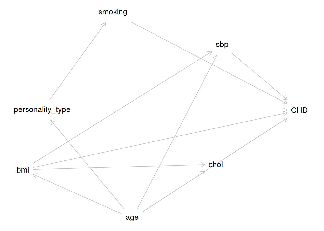
wcgs_dag <- dagitty(
  'dag {
    personality_type [exposure, pos="0,0"]
    CHD [outcome, pos="4,0"]
    age [pos="1.4,2"]
    bmi [pos="-0.3,1.1"]
    smoking [pos="1.1,-1.8"]
    chol [pos="2.7,1"]
    sbp [pos="2.8,-1.2"]

    personality_type -> CHD
    age -> CHD
    age -> chol
    age -> sbp
    age -> bmi
    age -> personality_type
    personality_type -> smoking
    smoking -> CHD
    chol -> CHD
    sbp -> CHD
    bmi -> CHD
    bmi -> chol
    bmi -> sbp
  }'
)

plot(wcgs_dag)

Figure 2: Directed Acyclic Graph (DAG) for the WCGS study. personality_type = personality type (exposure; Type A vs Type B); CHD = coronary heart disease events (outcome); chol = serum cholesterol; sbp = systolic blood pressure.

In Figure 2, age is a confounder: it has direct causal arrows to both the exposure (personality_type) and the outcome (CHD). We assume personality_type -> smoking rather than smoking -> personality_type as an explicit modeling assumption for this teaching example: we treat Type A behavior pattern as a relatively stable trait that can influence smoking behavior. Under that assumption, smoking is a mediator on the path personality_type -> smoking -> CHD, not a confounder. BMI is causally affected by age. Cholesterol and SBP are causally affected by both age and BMI. All three have direct effects on CHD. Unlike in HERS, where HT was randomized to estimate its causal effect on CHD event risk, we cannot assume the exposure is unconfounded here.

wcgs_adj <- adjustmentSets(
  wcgs_dag,
  exposure = "personality_type",
  outcome = "CHD",
  type = "minimal"
)
wcgs_adj
#> { age }

The adjustmentSets() function returns the minimal set(s) of variables that block all backdoor paths from personality_type to CHD. Adjusting for any of these minimal sets is sufficient to estimate the total causal effect of Type A behavior on CHD (under the assumptions encoded in the DAG).

7 Regression Adjustment

Under the causal assumptions (consistency, conditional exchangeability, and positivity), the causal effect can be estimated by adjusting for the confounders \(\tilde{L}\) in a regression model.

7.1 Direct standardization (G-computation)

The G-computation estimator (also called direct standardization or standardization) estimates the ATE by:

1. Fitting a regression model: \(\hat{\mu}(a, \tilde{l}) = \widehat{\text{E}{\left[Y \mid A = a, \tilde{L} = \tilde{l}\right]}}\)

2. Predicting the potential outcome mean for each individual under both treatment levels \(a = 1\) and \(a = 0\): \[\hat{Y}_i(a) = \hat{\mu}(a, \tilde{L}_i)\]

3. Averaging over the study population: \[\widehat{\text{E}{\left[Y(a)\right]}} = \frac{1}{n} \sum_{i=1}^n \hat{Y}_i(a)\]

4. Estimating the ATE as the contrast: \[\widehat{\text{ATE}} = \widehat{\text{E}{\left[Y(1)\right]}} - \widehat{\text{E}{\left[Y(0)\right]}}\]

G-computation is model-based: it relies on the regression model being correctly specified. A misspecified model will produce biased causal estimates even if confounders are included.

G-computation is easily generalized to:

• Binary outcomes (using logistic regression)
• Survival outcomes (using Cox or Weibull models)
• Multiple treatments or treatment levels

7.2 Regression adjustment in linear models

When the outcome is continuous and the regression model is linear, G-computation simplifies to the adjusted treatment coefficient from a linear regression:

\[Y = \beta_0 + \beta_A A + \tilde{\beta}_L \cdot \tilde{L} + \varepsilon\]

Under consistency, conditional exchangeability, and positivity, the coefficient \(\beta_A\) estimates the average causal effect of \(A\) on \(Y\) (the ATE, if the model is correctly specified and effect modification by \(\tilde{L}\) is absent).

The regression adjustment estimator for the ATE is equivalent to G-computation when the outcome model is linear and has no treatment-covariate interactions. When there are interactions, G-computation and regression adjustment can give different estimates. G-computation is preferred in that case.

7.3 Example: regression adjustment for LDL in HERS

The HERS study DAG (see Section 6.4) shows that LDL and HDL are mediators of the HT → CHD pathway. For estimating the total causal effect of HT on CHD, we should not adjust for LDL or HDL.

However, to estimate the causal effect of HT on LDL itself, we use a separate regression model with LDL as the outcome. In this model, LDL is no longer a mediator but the outcome of interest.

Since HT was randomized in HERS, no adjustment is needed for causal identification of HT → LDL. However, adjusting for strong predictors of LDL improves precision:

library(haven)
library(dplyr)

hers <- read_stata(fs::path_package("rme", "extdata/hersdata.dta"))

hers_ldl <-
  hers |>
  filter(!is.na(LDL)) |>
  mutate(
    HT = factor(HT, levels = c(0, 1), labels = c("Placebo", "HT")),
    statins = factor(statins, levels = c(0, 1), labels = c("No", "Yes")),
    diabetes = factor(diabetes, levels = c(0, 1), labels = c("No", "Yes"))
  )

library(gtsummary)

model_ldl_adj <-
  lm(LDL ~ HT + age + BMI + diabetes + statins, data = hers_ldl)

model_ldl_adj |>
  tbl_regression() |>
  bold_labels()

Table 7: Adjusted regression for the causal effect of HT on LDL in HERS. Since HT was randomized, adjustment is for precision only.

Characteristic	Beta	95% CI	p-value
HT
Placebo	—	—
HT	-0.14	-2.9, 2.6	>0.9
age in years	-0.23	-0.44, -0.02	0.035
BMI (kg/m^2)	0.46	0.19, 0.72	<0.001
diabetes
No	—	—
Yes	-4.6	-7.9, -1.4	0.005
statins
No	—	—
Yes	-17	-20, -14	<0.001
Abbreviation: CI = Confidence Interval

The estimated causal effect of HT on LDL is approximately −11 mg/dL (negative = lower LDL on HT), with narrower confidence intervals than the unadjusted estimate.

8 Propensity Score Methods

Propensity score methods are an alternative approach to confounding adjustment in observational studies. They replace adjustment for a high-dimensional confounder set \(\tilde{L}\) with adjustment for a single scalar summary: the propensity score.

Definition 15 (Propensity score) The propensity score is the conditional probability of treatment given the observed covariates: \[e(\tilde{L}) = \text{P}{A = 1 \mid \tilde{L}}\]

Rosenbaum and Rubin (1983) showed that if \(A \perp\!\!\!\perp (Y(0), Y(1)) \mid \tilde{L}\) (conditional exchangeability given \(\tilde{L}\)), then also: \[A \perp\!\!\!\perp (Y(0), Y(1)) \mid e(\tilde{L})\]

That is, the propensity score is a balancing score: conditioning on the propensity score is sufficient to remove confounding.

8.1 Propensity score estimation

The propensity score is estimated by fitting a model for the probability of treatment given covariates, typically using logistic regression:

\[\text{logit}(\hat{e}(\tilde{L}_i)) = \hat{\beta}_0 + \hat{\beta}_1 L_{i1} + \cdots + \hat{\beta}_p L_{ip}\]

The estimated propensity score \(\hat{e}(\tilde{L}_i)\) is the predicted probability of treatment for each individual.

8.2 Propensity score methods

There are four main ways to use the propensity score:

1. Matching: Match each treated individual to one or more untreated individuals with similar propensity scores. The matched dataset is then analyzed as a simple comparison.

2. Stratification (subclassification): Divide individuals into strata based on propensity score quantiles. Estimate the causal effect within each stratum, then combine across strata.

3. Inverse probability weighting (IPW): Weight each individual by the inverse of their probability of receiving the treatment they actually received. See Definition 16 below.

4. Covariate adjustment using the propensity score: Include the estimated propensity score as a covariate in a regression model for the outcome.

Definition 16 (Inverse probability weighting (IPW)) The inverse probability weighted (IPW) estimator of the ATE uses weights: \[w_i = \frac{A_i}{\hat{e}(\tilde{L}_i)} + \frac{1 - A_i}{1 - \hat{e}(\tilde{L}_i)}\]

The IPW estimator of \(\text{E}{\left[Y(a)\right]}\) is: \[\widehat{\text{E}{\left[Y(a)\right]}}_{\text{IPW}} = \frac{\sum_{i: A_i = a} w_i Y_i}{\sum_{i: A_i = a} w_i}\]

Reweighting by \(w_i\) creates a pseudo-population in which treatment is independent of covariates, effectively removing confounding.

8.3 Propensity score example: WCGS

In the WCGS study, we can use propensity score methods to estimate the causal effect of Type A behavior on CHD. We first fit a logistic regression model predicting Type A behavior from the confounders identified by the DAG (Section 6.7):

library(dplyr)

here::here() |>
  fs::path("Data/wcgs.rda") |>
  load()

wcgs_ps <-
  wcgs |>
  mutate(
    dibpat_A = as.integer(dibpat == "Type A"),
    chd69_yn = as.integer(chd69 == "Yes")
  ) |>
  filter(
    !is.na(age), !is.na(dibpat), !is.na(chd69),
    !is.na(bmi), !is.na(sbp), !is.na(chol), !is.na(smoke)
  )

ps_model <- glm(
  dibpat_A ~ age + bmi + sbp + chol + smoke,
  data = wcgs_ps,
  family = binomial()
)

wcgs_ps <- wcgs_ps |>
  mutate(
    ps = predict(ps_model, type = "response"),
    ipw = dibpat_A / ps + (1 - dibpat_A) / (1 - ps)
  )

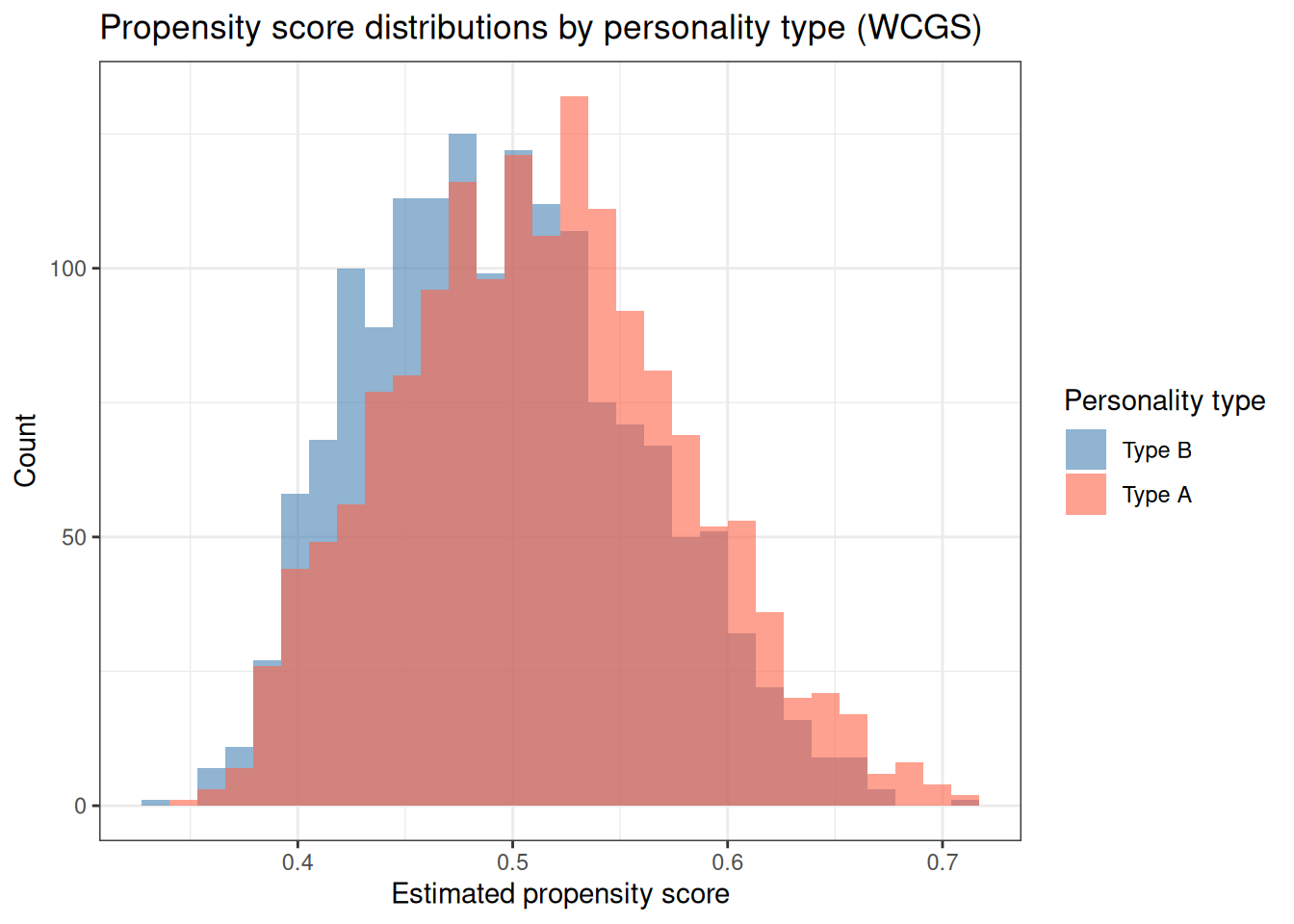
library(ggplot2)

ggplot(wcgs_ps, aes(x = ps, fill = factor(dibpat_A))) +
  geom_histogram(alpha = 0.6, bins = 30, position = "identity") +
  scale_fill_manual(
    values = c("steelblue", "tomato"),
    labels = c("Type B", "Type A"),
    name = "Personality type"
  ) +
  labs(
    x = "Estimated propensity score",
    y = "Count",
    title = "Propensity score distributions by personality type (WCGS)"
  ) +
  theme_bw()

Figure 3: Distribution of estimated propensity scores by personality type in the WCGS study. Good overlap between the two groups (the overlap or common support assumption) supports positivity.

library(gtsummary)

outcome_ipw <- glm(
  chd69_yn ~ dibpat_A,
  data = wcgs_ps,
  weights = ipw,
  family = quasibinomial()
)

outcome_ipw |>
  tbl_regression(exponentiate = TRUE) |>
  bold_labels()

Characteristic	OR	95% CI	p-value
dibpat_A	1.93	1.48, 2.53	<0.001
Abbreviations: CI = Confidence Interval, OR = Odds Ratio

The IPW-weighted odds ratio for Type A vs. Type B behavior estimates the causal odds ratio for CHD, adjusting for confounding by age, BMI, SBP, cholesterol, and smoking.

Compare this to the unadjusted estimate: the difference reflects the degree of confounding in the WCGS data.

9 Summary

Causal inference requires moving beyond statistical association to make statements about what would happen under intervention. The key ideas from this chapter are:

Potential outcomes define what we mean by a causal effect. For each unit, there is a potential outcome under treatment and a potential outcome under control; the individual causal effect is their difference.

Causal estimands — ATE, ATT, ATU — summarize the causal effect at the population level.

Three key assumptions are needed to identify causal effects from observed data:

1. Consistency: The observed outcome equals the potential outcome under the received treatment.
2. Exchangeability: Treatment assignment is independent of potential outcomes, given measured confounders.
3. Positivity: Every individual has a positive probability of receiving each treatment level.

Randomized experiments achieve unconditional exchangeability and allow unbiased causal inference from simple treatment comparisons.

In observational studies, confounding violates exchangeability. DAGs help identify which variables are confounders, mediators, and colliders, and the backdoor criterion identifies sufficient adjustment sets.

Estimation methods — regression adjustment (G-computation) and propensity score methods (matching, stratification, IPW) — can recover causal estimates under the three assumptions above.

Learning Objectives

After completing this chapter, students should be able to:

1. Define potential outcomes and the fundamental problem of causal inference.

2. Distinguish the ATE, ATT, and ATU, and explain when they agree and when they differ.

3. State and interpret the three core causal assumptions: consistency, exchangeability, and positivity.

4. Explain why randomization achieves unconditional exchangeability and allows unbiased causal effect estimation.

5. Use a DAG to identify confounders, mediators, and colliders, and apply the backdoor criterion to select sufficient adjustment sets.

6. Describe the G-computation estimator and explain how it relates to regression adjustment.

7. Describe propensity score methods (matching, stratification, IPW) and explain how they use the propensity score to remove confounding.

8. Contrast causal inference from randomized trials with causal inference from observational studies, and articulate the additional assumptions required in each setting.

References

Hernán, Miguel A., and James M. Robins. 2020. Causal Inference: What If. Chapman & Hall/CRC. https://www.hsph.harvard.edu/miguel-hernan/causal-inference-book/.

Holland, Paul W. 1986. “Statistics and Causal Inference.” Journal of the American Statistical Association 81 (396): 945–60. https://doi.org/10.2307/2289064.

Hulley, Stephen, Deborah Grady, Trudy Bush, et al. 1998. “Randomized Trial of Estrogen Plus Progestin for Secondary Prevention of Coronary Heart Disease in Postmenopausal Women.” JAMA : The Journal of the American Medical Association (Chicago, IL) 280 (7): 605–13.

Rosenbaum, Paul R., and Donald B. Rubin. 1983. “The Central Role of the Propensity Score in Observational Studies for Causal Effects.” Biometrika 70 (1): 41–55. https://doi.org/10.1093/biomet/70.1.41.

Rosenman, Ray H, Richard J Brand, C David Jenkins, Meyer Friedman, Reuben Straus, and Moses Wurm. 1975. “Coronary Heart Disease in the Western Collaborative Group Study: Final Follow-up Experience of 8 1/2 Years.” JAMA 233 (8): 872–77. https://doi.org/10.1001/jama.1975.03260080034016.

Rubin, Donald B. 1974. “Estimating Causal Effects of Treatments in Randomized and Nonrandomized Studies.” Journal of Educational Psychology 66 (5): 688–701. https://doi.org/10.1037/h0037350.

Vittinghoff, Eric, David V Glidden, Stephen C Shiboski, and Charles E McCulloch. 2012. Regression Methods in Biostatistics: Linear, Logistic, Survival, and Repeated Measures Models. 2nd ed. Springer. https://doi.org/10.1007/978-1-4614-1353-0.