Supplementary Analysis

This notebook contains supplementary analyses referenced in the main manuscript. Results computed here are embedded in the HTML version of the article.

Data exploration

In [1]:

head(mtcars)

In [2]:

First six rows of the example dataset.

Additional models

In [3]:

fit <- lm(mpg ~ wt + hp, data = mtcars)
summary(fit)
#> 
#> Call:
#> lm(formula = mpg ~ wt + hp, data = mtcars)
#> 
#> Residuals:
#>    Min     1Q Median     3Q    Max 
#> -3.941 -1.600 -0.182  1.050  5.854 
#> 
#> Coefficients:
#>             Estimate Std. Error t value Pr(>|t|)    
#> (Intercept) 37.22727    1.59879  23.285  < 2e-16 ***
#> wt          -3.87783    0.63273  -6.129 1.12e-06 ***
#> hp          -0.03177    0.00903  -3.519  0.00145 ** 
#> ---
#> Signif. codes:  0 '***' 0.001 '**' 0.01 '*' 0.05 '.' 0.1 ' ' 1
#> 
#> Residual standard error: 2.593 on 29 degrees of freedom
#> Multiple R-squared:  0.8268, Adjusted R-squared:  0.8148 
#> F-statistic: 69.21 on 2 and 29 DF,  p-value: 9.109e-12

In [4]:

par(mfrow = c(2, 2))
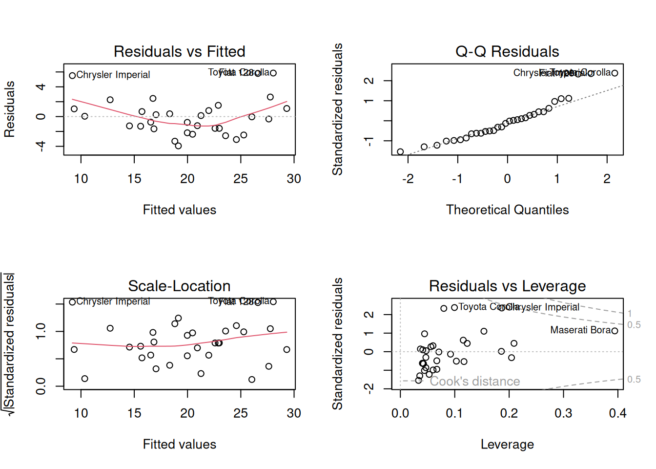
plot(fit)

Residual diagnostics for the supplementary regression model.